4. Model evaluation
In this section we will deal with the question how the performance of a model can be estimated. Special emphasis is put on the generalisability of models, and an evaluation technique which is commonly used in the field of pattern classification is adapted to suit our categorisation model. Finally, a note is made on chance-level performance of models.

For practical reasons only a very limited set of stimuli can be used in a perception experiment. Nevertheless, one wants to make claims about the general validity of the model. In Fukunaga and Kessell (1971) and Fukunaga (1972) a statistical method is presented for estimating the generalisable GOF of crisp categorisation models. A crisp categorisation model is defined as a categorisation model which has deterministic representation and retrieval stages and which generates class probability vectors which always contain N_r - 1 components equal to zero and one component equal to one. Fuzzy categorisation models like our model, on the other hand, are defined as models which generate output probabilities that can take on any value between zero and one. We will briefly review the evaluation method for the crisp case

below and extend it to fuzzy classification models.

First we need to introduce some new notation. Let us indicate a categorisation model by , which stands for a vector of model parameters. Furthermore, we define a data set as a set of vector pairs , where and are the feature vector and response vector for a stimulus S_i. The term testing is defined as determining the GOF of a trained model on a (possibly new) set of data. Finally, let indicate the probability that the model , which is trained on a data set , makes an incorrect categorisation of a datum from the test set .

The experimenter aims to estimate the performance of a certain categorisation model on a general data set . In other words, ideally, the experimenter wants to measure (the entire set is used as training set as well as test set). In general, however, only a representative subset of is available. In Fukunaga and Kessell (1971) and Fukunaga (1972) it is shown that lower and upper bounds for can be estimated from . This is expressed in the inequality

(24)

where E{x} denotes the expected value of a quantity x.

The lower bound can be simply estimated by training and testing the model on the entire data set produced in an experiment. Thus we replace by . The upper bound can be estimated using a cross validation technique. In a cross validation technique the training set and test set are disjunct: .

The two best-known cross-validation methods are the "sample partitioning" method and the "Leaving-One-Out" (LOO) method. In the sample partitioning method, the N available data are subdivided into two or more distinct subsets, and the model is trained on all but one subsets and tested on the remaining subset. In order to get accurate estimates of both the model and the GOF of the model, the training sets as well as the test set must be sufficiently large. As this is often not the case for perception data, this method may not lead to accurate estimates of GOF. In the case that N is not large, the LOO-method can be used, which is computationally more expensive but gives more accurate GOF estimates. In this method, the N data are subdivided into 2 subsets, one containing N - 1 data and the other subset containing the single remaining datum. The model is trained on the N - 1 data and tested on the remaining datum. Next, the N data are again subdivided into 2 subsets, one containing N - 1 data and the other subset containing a different remaining datum. Again, a model is trained and tested as before, and the process is carried out N times in total, leaving out each of the N data once in the process. The resulting test error is defined as the average of the N test errors. As each datum is effectively used as training as well as test item, the method can be shown to make optimal use of the available samples, that is, it gives the closest possible upper bound approximation , given a set of N data (Fukunaga, 1972).

4.1 The LOO-method for fuzzy classification
The method for estimating described above was developed for crisp categorisation models. It can, however, be easily generalised to suit fuzzy categorisation models, like our SLP-based model.

In crisp classification the generally preferred GOF-measure is the rate of correct classification, or percentage correct, P_c, with associated BOF-measure percentage incorrect . In fuzzy classification, such as for human classification models, a number of measures of GOF and BOF are used, such as the sum-of-squared-errors (SSE) and the G² statistic (e.g. ten Bosch and Smits, 1996; Nosofsky and Smith, 1992). Whichever measure of BOF is preferred, it can replace the probability of an incorrect classification p.e. in Eq. (24).

4.2 Chance-level performance
When the performance of a model is evaluated, it is important to be aware of the chance-level performance of the model. The chance-level performance is here defined as the highest possible goodness-of-fit that can be obtained without any knowledge of the stimulus features. This means that, at the output of the chance-level model, we find a fixed class probability vector which does not depend on the stimulus. Note that the chance-level model can be represented by a single-layer perceptron (SLP) in which all weights connecting the stimulus features to the output nodes are zero and only the biases are nonzero. Given a particular stimulus-response matrix, chance level can thus be calculated simply by using the same estimation technique which is used for the actual model estimations.

5. Example
In this section, the developed methodology is illustrated by a practical example. The data in this example are part of a much larger data set that is used for a phonetic research project which is published elsewhere (Smits et al. 1995a, 1995b).

In this section model estimation and evaluation will sometimes be referred to as training and testing, respectively.

5.1 Perception experiment
The purpose of the research published in Smits et al. (1995a, 1995b) was to assess the perceptual relevance of various acoustic features for the perception of the stop consonants /b, d, p, t, k/. A subset of the stimuli consisted of short acoustic segments, the "release bursts", which were excised from natural utterances consisting of an unvoiced stop consonant (/p/, /t/ or /k/) followed by a vowel (/a/, /i/, /y/ or /u/). These stimuli were presented to subjects who responded to each presentation with either P, T, or K (N_r = 3). In total 24 stimuli (2 tokens x 3 consonants x 4 vowels) were used (N_s = 24). Each stimulus was presented 6 times to each of 20 subjects. The responses of all subjects were summed, yielding a total of 120 responses per stimulus (N_p = 120).

5.1.1 Stimulus features
On the basis of a number of phonetic studies (e.g. Blumstein & Stevens, 1979) it was decided to measure the following 5 stimulus features on each of the 24 stimuli:

1. Energy of the burst (E);
2. Length of the burst (L_e);
3. Global spectral tilt of the burst (T);
4. Frequency of a broad mid-frequency peak of the burst (Fr);
5. Height of the broad mid-frequency peak of the burst (H).

The specific methods for measuring these features are described in Smits et al. (1995b). Note that these stimulus features were not explicitly controlled in the stimulus set, because the stimuli were excised portions of naturally uttered speech.

The stimulus features were converted to Z-scores using Eq. (7).

5.2 Model estimation
In order to establish what subset of the 5 proposed features gave the best account of the observed classification behaviour, all possible subsets of 1 to 4 features were tried. Thus, various SLP topologies were trained and tested on the data: SLPs with 1, 2, 3, or 4 input nodes. For all topologies the number of output nodes was 3. Ideally, we would have trained and tested each model on all possible subsets of stimulus features to assess which set gives the best generalisable account of the data. However, as the computing cost of the LOO-method is very high we adopted the following less expensive method. Each model having N_F input nodes (N_F = 1,2,3,4) was trained on all possible subsets of N_F features. The 3 subsets that gave the best GOF-train were then used for cross validation using the LOO-method. Finally, the feature subset which resulted in the best GOF-test was selected as the overall best subset of N_F features, given the model topology.

The GOF-measure P_c that was maximised in our model estimations - and in which the results will be expressed - is defined by:

(25)

Note that .

P_c is interpreted as the average probability of the model's generating the observed response on a single presentation of a randomly selected stimulus. For the sake of simplicity, we will interpret P_c as the probability of a correct response, hence the subscript "c".

For further details on the GOF-measure and the model estimation technique the reader is referred to Smits (1995) and Ten Bosch and Smits (1996).

5.3 Model evaluation
Chance level for the observed stimulus-response matrix was 62.1%. Chance level was calculated by performing a model estimation using no input nodes, only one bias node (thus 3 bias parameters were estimated, 1 of which was fixed at value 1). While the marginal distribution of the stimulus-response matrix is (0.387, 0.213, 0.400) for the response classes P, T and K, respectively, the chance-level model has fixed output probabilities (0.481, 0.225, 0.294).

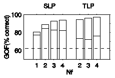
The GOF-levels for training and testing of the various model topologies are listed in Table 2 and are shown graphically in Figure 5. Table 2 also lists the number of parameters N_w for each topology.

Table 2. Goodness of fit on training and testing for various model fits in %.

NF	1	2	3	4
Nw	6	9	12	15
GOF train	80.7	88.7	92.8	93.8
GOF test	77.5	84.6	83.0	82.3
Chance level	62.1	62.1	62.1	62.1

With increasing number of parameters, GOF-train keeps increasing. GOF-test on the other hand, quickly reaches a maximum with increasing number of parameters, and then slowly decreases. This is a typical example of overfitting (e.g. Haykin, 1994). In general, overfitting, or non-generalizability, occurs when the number of model parameters is in the order of - or larger than - the number of data. For our example the number of degrees of freedom of the data is (N_r - 1)N_s = 48. Apparently, we need to keep the number of model parameters in our example roughly below 1/4 of the number of degrees of freedom of the data in order to make a generalisable model estimation.

5.4 Model interpretation
Let us look more closely at the model fit with the highest GOF-test, that is, the SLP with 2 input nodes. GOF-train and GOF-test are 88.7 and 84.6, respectively. The optimal stimulus features for this model are the burst energy E and the height of the mid-frequency peak H. The model parameters are w₁₁ = -2.447, w₁₂ = 0.016, w₁₃ = -0.670, w₂₁ = -1.483, w₂₂ = -0.893, w₂₃ = 1.373, b₁ = -2.721, b₂ = -3.284, b₃ = -2.488, which leads to response regions for "P", "T", and "K" defined as:

P:

(26)

T:

(27)

K:

(28)

Don't-know regions for the various class pairs are defined as:

P-T: -1.122E - 1.188H - 3.003 > 5

(29)

P-K: -1.559E - 0.006H - 2.605 > 5

(30)

T-K: - 0.343E + 0.240H - 2.886 > 5

(31)

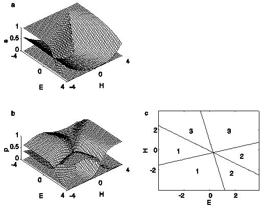
Figure 6a shows the functions s₁, s₂, s₃ and Figure 6b shows the associated class probabilities p₁, p₂, p₃. Figure 6c shows the equal-probability class boundaries as defined in Eqs. (26-28) (solid straight lines), the approximate stimulus region (enclosed by circle), defined as the region in which all points are less than two standard deviations away from the origin, and the boundaries of the don't-know regions as defined in Eqs. (29-31) (dashed lines).

Figure 6. 6a: The functions s₁, s₂, s₃ as function of the stimulus features E and H for the SLP with the highest GOF-test. 6b: The functions p₁, p₂, p₃ as function of the stimulus features E and H for the same model. 6c: The equal-probability boundaries between classes 1 ("P"), 2 ("T") and 3 ("K") (solid straight lines), the stimulus region (circle) and the boundaries of the don't-know regions (dashed lines).

With respect to the don't know regions we find that they all lie outside the stimulus region. Concerning the response regions, we roughly find that subjects tend to respond "P" (class 1) to stop-consonant release bursts when they have low energy and a weak mid-frequency peak. Bursts with high energy and a weak mid-frequency peak are labelled "T" (class 2), and bursts with a strong mid-frequency peak are generally labelled "K" (class 3). (Recall that all stimulus features were transformed to Z-scores, so almost all feature values lie within the range [-2,2].) These findings are in agreement with the results of earlier phonetic studies in which acoustic classification experiments were carried out, like Halle, Hughes, & Radley (1957) and Blumstein & Stevens (1979), as well as the results of phonetic perception studies where synthetic stimuli were used, like Blumstein & Stevens (1980) and Kewley-Port, Pisoni & Studdert-Kennedy (1983).

Back to Publications

Back to Phonetics and Linguistics Home Page