Let us look at a number of examples in the simplest situation of interest: one feature and two classes. We start by noting that when the feature space is one-dimensional the feature weights for the two classes can have either the same sign or opposite sign, which corresponds to the s-functions of the two classes being "pointed" in either the same direction or in opposite direction. These two situations lead to very different model behaviour.
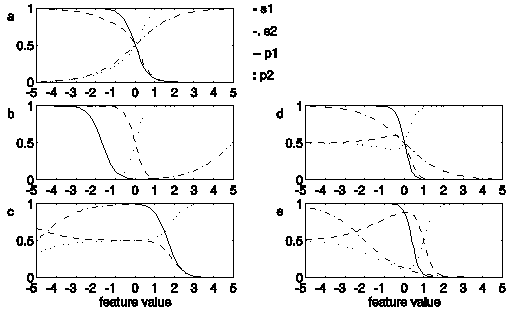
Figure 3. The functions s1 (solid line),
s2 (dash-dotted line), p1
(dashed line) and p2 (dotted line) as function
of the stimulus feature for five examples of the SLP. The parameter
values are: Figure 3a: w1 = -3, w2
= 1, b1 = b2 = 0. Figure
3b: w1 = -3, w2 = 1, b1
= b2 = -5. Figure 3c: w1 =
-3, w2 = 1, b1 = b2
= 5. Figure 3d: w1 = -5, w2
= -1, b1 = b2 = 0. Figure
3e: w1 = -5, w2 = -1, b1
= 2, b2 = -2.
Figure 3a shows the s-functions (continuous line and dash-dotted
line) and the class-probability functions (dashed line and dotted
line) for a hypothetical basic situation for a model with 1 feature
and 2 classes. The parameters for this model have been chosen
to have the following values: w1 = -3, w2
= 1, b1 = b2 = 0. The
class boundary is located at F = 0.
In Figure 3b, exp(- ) is increased by decreasing both
biases to -5, while keeping w1 and w2
unchanged. As the scaling factor exp(-) increases,
the class-probability functions have become steeper, while the
location of the class boundary is unchanged. In the region directly
around the class boundary, where both s-functions are close
to 0, case 1 applies.
) is increased by decreasing both
biases to -5, while keeping w1 and w2
unchanged. As the scaling factor exp(-) increases,
the class-probability functions have become steeper, while the
location of the class boundary is unchanged. In the region directly
around the class boundary, where both s-functions are close
to 0, case 1 applies.
In Figure 3c exp(-) is decreased, compared to Figure
3a, by increasing both biases to +5, while w1
and w2 have again been unchanged. Case 2 now
applies in the region directly around the class boundary, where
both s-functions are close to 1. Here the model is more
or less constant and both class probabilities are roughly equal
to 0.5. As  is still the same as in Figures 3a and
b, the class boundary is still located at F = 0.
is still the same as in Figures 3a and
b, the class boundary is still located at F = 0.
The parameters for Figure 3d are the same as those for Figure
3a, except that has now been manipulated by decreasing
both w1 and w2 by an amount
of -2, resulting in w1 = -5, w2
= -1. Note that both sigmoids are now pointed in the same direction.
As has been unaffected, the location of the class
boundary is unchanged. For large feature values both s-functions
are close to zero, leading to a case-1 situation. For negative
feature values of large magnitude both s-functions are
close to 1, leading to a case-2 situation. Both probability functions
flatten off to a value of 0.5. Interestingly, both probability
functions have a local extremum at approximately F = 0.3.
Note that, while s1 and s2
are monotonically decreasing functions, p1 is
increasing for small values of F and p2
is increasing for large values of F. In Figure 3e the size
of the extremum is somewhat blown up by changing the biases to
b1 = -5, b2 = -1. Note that
the location of the class boundary has shifted.
In appendix 2 it is demonstrated that the existence of local extrema is not restricted to models in a one-dimensional feature space, but can instead occur in a feature space of any dimension. Furthermore, the proof shows that the weight vectors for the different
classes are not required to be parallel for an extremum to exist, nor does a class need to be "enclosed" by competing classes in order to have a local extremum. Figure 4 illustrates these properties for a 2-feature, 3-class model.
Figure 4. The functions s1, s2,
s3 (Figure 4a) and class probabilities p1,
p2, p3
(Figure 4b), for one example of the SLP. The parameter values
are: w11 = 0, w21 = 2, w12
= 2, w22 = 2, w13 = 2, w23
= 0, b1 = -4, b2 = 0, b3
= -4. x and y are the stimulus features.
The model parameters are b1 = -4, b2
= 0, b3 = -4, and w11 = 0,
w21 = 2, w12 = 2, w22
= 2, w13 = 2, w23 = 0. Figure
4a shows the functions s1, s2
and s3, while Figure 4b shows the corresponding
probability functions p1, p2
and p3. Note that the class-2 probability
surface exhibits a pronounced local maximum.
Let us summarise and discuss the findings of this section. First
of all, we have found it useful to separate the average component
and the differential component in the
ratio of the response probabilities for 2 classes.
exclusively determines the location of the equal-probability boundary
between the two classes. This class boundary is linear in F.
The effect of is one of "scaling" the contribution
of . Two extreme cases of scaling have been examined.
In the first case is negative of large magnitude. In an
important instance of this case, when all biases approach  , the SLP-based model has been shown to coincide with
a SCM which has all the class prototypes located at infinite distance
from the origin of the feature space. What is the psychological
significance of this finding? Arguing from the angle of the asymptotic
SCM, two possible psychological mechanisms which are compatible
with this type of model behaviour suggest themselves. Firstly,
subjects may base the classification of an incoming stimulus on
a comparison with idealised prototypes, that is, prototypes which
not so much lie infinitely far away, but simply lie outside the
confined region in the feature space that contains all stimuli.
Alternatively, subjects may base their classifications on a comparison
with class boundaries, rather than class prototypes.
, the SLP-based model has been shown to coincide with
a SCM which has all the class prototypes located at infinite distance
from the origin of the feature space. What is the psychological
significance of this finding? Arguing from the angle of the asymptotic
SCM, two possible psychological mechanisms which are compatible
with this type of model behaviour suggest themselves. Firstly,
subjects may base the classification of an incoming stimulus on
a comparison with idealised prototypes, that is, prototypes which
not so much lie infinitely far away, but simply lie outside the
confined region in the feature space that contains all stimuli.
Alternatively, subjects may base their classifications on a comparison
with class boundaries, rather than class prototypes.
In the second case of extreme scaling is large. In
this situation the response probabilities for the two classes
involved are approximately equal and independent of F.
This may be accompanied by the existence of a local extremum for
the probability functions for both classes elsewhere in the feature
space. What is the psychological significance of these findings?
First of all, the SLP-based model apparently allows for the existence
of extensive "don't-know" regions in the feature space,
where the precise stimulus composition is irrelevant and the subject
is guessing. Secondly, we have found that, although the SLP is
based on a processing of stimulus features through monotonic sigmoid
functions, the actual response probability functions may in some
cases be non-monotonic and may only reach substantial values in
a localised region of the feature space. Thus the model's output
nodes (after choice rule) can indeed be said to have "localised
receptive fields", meaning that the nodes' output reaches
high values only for a bounded stimulus range (compare Kruschke,
1992, p. 34). Obviously, this model property - as well as the
previously discussed ones - is brought about by the application
of the choice rule, and does not hold for the "bare"
SLP.
3.3 Model interpretation
Based on the observations of the previous section we propose that
the interpretation of the model should be based primarily on studying
the model's class boundaries. As demonstrated in section 5, as
well as elsewhere (Smits et al, 1995b), such boundary-based
interpretation can provide valuable insight in psychological processes
such as the classification of speech sounds. For feature spaces
of dimension 1 or 2, such interpretation may be guided by a visual
as well as a mathematical representation of the boundaries. For
feature spaces of higher dimensions, however, a visual interpretation
is difficult or impossible, but the linear boundary equations
remain readily interpretable (Smits et al, 1995b). Obviously,
all class boundaries can be derived by calculating
for all possible pairs of classes.
Furthermore, it may be interesting to investigate the occurrence
of significant "don't-know" regions within the stimulus
region of the cue space. Some basic manipulations show that the
condition expressed in Eq. (18) is approximated when both dm(F)
and dn(F) are larger than a certain
number, say  . Note that
  if we choose
  . Establishing the region
of F where all dj are larger than
will identify the area in the feature space which
contains stimuli that subjects find hard to identify, if such
an area is present at all.
. Establishing the region
of F where all dj are larger than
will identify the area in the feature space which
contains stimuli that subjects find hard to identify, if such
an area is present at all.
If we apply these interpretation strategies to the example of
Figure 4, we find the following response regions:
class 1: 
|
(20) |
class 2: 
|
(21) |
class 3: 
|
(22) |
where  and
and  represent
the 2 feature dimensions.
represent
the 2 feature dimensions.
The don't-know region is defined by:

|
(23) |
the tip of which is just visible in the right-hand corner in Figure 4.
 Back to SHL 9 Contents
 Back to Phonetics and Linguistics Home Page
