3.1 Mathematical definitions
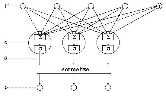
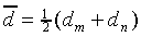
The SLP is the core of our categorisation model. It is used to model the retrieval stage, that is, the mapping of stimulus features to class probabilities. The structure of the SLP used in our model is shown schematically in Figure 2.

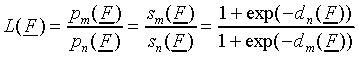
Figure 2. Schematic representation of the SLP as it is used in our model. The top row of small circles represents the input layer including the bias. The middle row of large circles represents the output layer. The symbols and represent summation and sigmoid transformation, respectively. For further explanation see text.

Up to application of the choice rule (Eq. 6), the expressions in this section are common knowledge in the perceptron literature (e.g. Lippman, 1987; Hertz, Krogh and Palmer, 1991; Haykin, 1994), and are repeated here simply for the sake of definition.

The SLP consists of an input layer and an output layer and no hidden layers. The stimulus features are clamped to the input nodes, represented as the top row of circles in Figure 2. The input nodes pass the features unchanged. One input node is assigned to each stimulus feature. The SLP in Figure 2 has 4 input nodes. The top right circle with the number "1" is the bias node. Instead of transferring a feature value, this node simply outputs a fixed value 1.

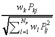
All input nodes, including the bias node, are connected to all output nodes. A weight is associated with each connection. The feature value passing through the connection is multiplied by the respective weight before reaching the output node. The weights are the parameters of the model. The number of weights N_w, including biases, in the SLP equals

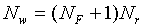
(3)

In the output nodes two processing steps take place. First, the weighted feature values of stimulus S_i are summed, yielding a quantity :

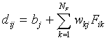
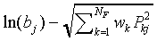
(4)

where is the bias, which is the weight between the bias node and output node j, and is the weight between input node k and output node j.

Next, d_ij is passed through a sigmoid activation function yielding a quantity s_ij defined by

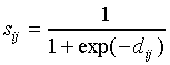
(5)

Note that , and and .

Finally, using Luce's (unbiased) choice rule (Luce, 1963), the outputs s_ij of the output nodes are normalised, yielding the quantity p_ij:

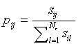
(6)

Note that this normalisation step is not traditionally part of the SLP.

The p_ij can now be interpreted as probabilities because and . The probabilities p_ij are interpreted as the probability that the model responds with class C_j when it is presented with stimulus S_i.

Generally, before being used as model input, the set of values for each feature is standardised over all stimuli using

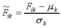
(7)

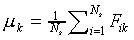where F_ik and are the original and standardised values of feature k of stimulus S_i, and and .

3.2 Model properties
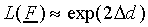
In this section we propose some simple mathematical manipulations which enable us to describe some properties of the SLP-based model and interpret a given set of model parameters. For this purpose we examine the ratio L(F) of the probability p_m(F) of responding class C_m and the probability p_n(F) of responding class C_n in the SLP:

(8)

In some of the derivations below we will drop the argument F to keep the expressions more transparent. Let us decompose the functions d_m and d_n into an average component and a differential component :

(9)

(10)

where

(11)

(12)

Now Eq. (8) can be rewritten as

(13)

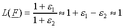
Let us study expression (13). We will first concentrate on . An important concept in categorisation models is the category boundary. The equal-probability boundary B_mn between classes C_m and C_n is defined as the subspace of where the ratio of probabilities of responding class C_m and C_n (8) equals unity:

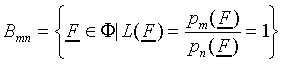
(14)

Using Eq. (13), the expression for the boundary B_mn reduces to

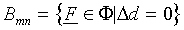
(15)

Thus we find that exclusively determines the location of the equal-probability boundary B_mn. Furthermore, as is a linear function of F, Eq. (15) states that the equal-probability boundary between any two classes is linear in the SLP-based categorisation model. It has been reported by others (e.g. Haykin, 1994; Lippman, 1987), that the "bare" SLP (without the choice rule) supports linear class boundaries. Eq. (15) shows that this still holds when the choice rule is applied.

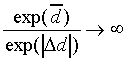
We now turn to . The factor exp(- ) in the numerator and denominator of Eq. (13) can be considered to "scale" the effect of , without discriminating between the two classes. Although has no influence on the shape and position of the class boundaries, its effect on the shape of the class-probability functions can be considerable. Two extreme cases of scaling can occur.

Case 1, the first extreme case, occurs when exp(- ) is much smaller than both and , that is, when

(16)

We can omit the terms "1" in Eq. (13) and the scaling factors exp(- ) in numerator and denominator cancel, which leads to

(17)

Note that condition (16) is equivalent to letting both d_m and d_n approach , or letting s_m and s_n approach 0 (using 8).

In appendix 1 it is proved that in a subset of situations where case 1 holds, namely when all biases approach minus infinity, the SLP-based model coincides with a special case of the SCM, in which the class prototypes are infinitely far away from the origin of the feature space. The relations between the various parameters in the two models for this case are listed in Table 1.

Table 1. The correspondence between SLP-parameters and SCM-parameters in the limit case .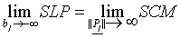

SLP parameters	Corresponding function of SCM parameters
bj
wkj

It may seem strange to express one infinite-valued parameter in another. Naturally, however, the listed relations approximately hold when the SLP-biases are finite negative numbers of large magnitude and the prototypes lie far - but not infinitely far - away from the origin.

Case 2, the second extreme case of scaling, occurs when exp( ) is much larger than both exp() and exp(-), that is, when

(18)

This leads to

(19)

Condition (18) is equivalent to letting both d_m and d_n approach , or letting s_m and s_n approach 1 (see Eq. 8).

Back to Publications

Back to Phonetics and Linguistics Home Page