Speech Filing System
How To: Use HTK Hidden Markov modelling toolkit with SFS
This document provides a tutorial introduction to the use of SFS in combination with the Cambridge Hidden Markov modelling toolkit (HTK) for pattern processing of speech signals. The tutorial covers installation, file conversion, phone and phone-class recognition, phonetic alignment and pronunciation variation analysis. This tutorial refers to versions 4.6 and later of SFS with version 3.3 of HTK.
Contents
- Installation
- Phone-class recognition
- Phone recognition
- Word recognition
- Phone alignment
- Pronunciation variation analysis
- Dysfluency recognition
1. Installation
These installation instructions refer to Windows computers. However most of the tutorial applies to other platforms where HTK and SFS command-line programs can be run under a Unix-like shell program.
Installation of CYGWIN
CYGWIN provides a Unix-like programming environment for Windows computers. We will use this environment in the tutorial so that we can write scripts for processing multiple files using the BASH shell language. This is useful because the shell language is simple yet powerful and runs on many different computing platforms.
CYGWIN can be downloaded from the CYGWIN home page at www.cygwin.com. From there download and run the program setup.exe which manages the installation of CYGWIN. This program first collects
information about your nearest CYGWIN distribution site then presents you with a list of components to install. Finally it downloads and installs the selected components. The same program can be used to update your installation as new software versions become available and to add/delete components. The setup program goes through these steps:
- Choose installation type. Choose "Install from Internet" if you have a reliable internet connection. Otherwise choose "Download from Internet" to copy the files onto your computer and then "Install from Local Directory" to install them.
- Choose installation directory. I suggest you leave this as "C:/cygwin" unless you know what you are doing.
- Select local package directory. Put here a directory (aka "folder") where CYGWIN will put the downloaded files before installation. You could enter a temporary directory name. I use "C:/download/cygwin". You may need to make the folders first using Windows Explorer.
- Select Internet connection. Leave as default.
- Choose a download site. Highlight an address in the list that seems to come from your own country. I choose "ftp://ftp.mirror.ac.uk/".
- Select packages. Use this page to investigate what packages (components) are available for download. Many are rather old and obscure elements of the Unix operating system. For the purposes of this tutorial you should download at least the following:
- All components in the "Base" category.
- Devel|BINUTILS: The GNU assembler, linker and binary utilities
- Devel|GCC: C Compiler
- Devel|GCC-G++: GCC C++ compiler
- Devel|MAKE: the GNU version of the 'make' utility
But feel free to install any of the other goodies that take your fancy.
- Download. The program then downloads and installs the selected packages.
- Installation complete. Choose both boxes to put a CYGWIN icon on your desktop and put a CYGWIN entry in the Start Menu.
After installation your should see a CYGWIN icon on the desktop and a Start menu option Start|Programs|Cygwin|Cygwin BASH shell. Either of these will start up a command window which provides a Unix-like environment in which we will be demonstrating SFS and HTK.

|
A good introduction to programming the Unix environment can be found in the old but essential "The Unix Programming Environment" by Kernighan and Pike. Available at Amazon.co.uk. |
It is worth exploring the CYGWIN environment to get used to the way it maps the names of the windows disks and folders. A folder like "C:\WINDOWS" is referred to as "c:/windows" in CYGWIN, or as "/cygdrive/c/windows". Your home directory in CYGWIN (referred to as "~") will actually be a subdirectory of the windows folder c:\cygwin\home.
Installation of a Text Editor
You will need a suitable text editor for editing scripts and other text files in this tutorial. My recommendation is TextPad which can be downloaded from www.textpad.com. This is a shareware program which requires registration if you use it extensively.
Installation of HTK
The Cambridge University Hidden Markov modelling toolkit (HTK) can be downloaded from htk.eng.cam.ac.uk. To check that you have read the licence conditions, they ask you first to register your name and e-mail address with them. They will then send you a password to use to download the HTK sources from http://htk.eng.cam.ac.uk/download.shtml. For the purposes of this tutorial I downloaded HTK−3.3.tar.gz into my cygwin home directory. By the time you read this tutorial it is very likely that there will be a new release with a different filename. The CYGWIN command to unpack this is just:
$ tar xvfz HTK-3.3.tar.gz
When unpacked, a sub-directory called "htk-3.3" will be created under your home directory. You can now delete the downloaded distribution file.
To build HTK for CYGWIN you first need to set a number of environment variables. I suggest you create a file called "htk.env" in your home directory containing the following:
export HTKCF='-O2 -DCYGWIN' export HTKLF='-o a.out' export HTKCC='gcc' export HBIN='..' export Arch=ASCII export CPU=cygwin export PATH=~/htk-3.3/bin.i686:$PATH |
Then each time you want to use HTK you can just type
$ source ~/htk.env
Alternatively you can put these commands in a file ".bash_login" in your home directory so that they will be executed each time you log in.
The first task is to configure HTK. The default destination directory for the HTK programs is in /usr/local/bin.i686, but you can change the direcory at configuration time. Run this command to set the destination directory to be ~/htk-3.3/bin/i686:
$ source ~/htk.env
$ cd ~/htk-3.3
$ ./configure --prefix=`echo ~/htk-3.3`
Unfortunately, as of the date of writing this tutorial, the HTK distribution needs patching before it can be compiled under CYGWIN. These are the follwing edits that you need to make using a text editor:
- Edit HTKLib/makefile and change the macro line CFLAGS to:
CFLAGS = -Wall -Wno-switch -g -O2 -I. -DCYGWIN -DARCH=ASCII
- Edit HTKTools/makefile and remove the reference to "-lX11" in the instructions for HSLab:
HSLab: HSLab.c $(HTKLIB)
	if [ ! -d $(bindir) ] ; then mkdir $(bindir) ; fi
	$(CC) -o $@ $(CFLAGS) $^ $(LDFLAGS)
	$(INSTALL) -m 755 $@ $(bindir)
We can now make HTK with the following instructions:
$ cd ~/htk-3.3
$ mkdir bin.i686
$ cd HTKLib
$ cp HGraf.null.c HGraf.c
$ cd ..
$ make
Installation of SFS
SFS can be downloaded from www.phon.ucl.ac.uk/resource/sfs/. Run the installation package and select the option "Add SFS to command-line path" to add the SFS program directory to the search path for programs to run from the command prompt and the CYGWIN shell. You may need to reboot for this change to take effect.
2. Phone-class recognition
In this section we will describe a "warm-up" exercise to show how SFS and HTK can be used together to solve a simple problem. The idea is to demonstrate the software tools rather than to achieve ultimate performance on the task.
We will demonstrate the use of SFS and HTK to build a system that automatically labels an audio signal with annotations which divide the signal into regions of "silence", "voiced speech", and "voiceless speech".
Source data
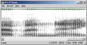
For this demonstration we will use some annotated data that is part of the SCRIBE corpus (see www.phon.ucl.ac.uk/resource/scribe). This data is interesting because it contains some "acoustic" level annotations - that is phonetic annotation at a finer level of detail than normal. In particular the annotation marks voiced and voiceless regions within phonetic segments. An example is shown in Figure 2.1.
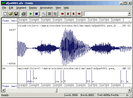
Figure 2.1 - Acoustic level annotations
The files we will be using are from the 'many talker' sub-corpus and are as follows
| Speaker | Training | Testing | ||
|---|---|---|---|---|
| Signal | Label | Signal | Label | |
| mac | acpa0002.pes acpa0003.pes acpa0004.pes |
acpa0002.pea acpa0003.pea acpa0004.pea |
acpa0001.pes | acpa0001.pea |
| mae | aepa0001.pes aepa0003.pes aepa0004.pes |
aepa0001.pea aepa0003.pea aepa0004.pea |
aepa0002.pes | aepa0002.pea |
| maf | afpa0001.pes afpa0002.pes afpa0004.pes |
afpa0001.pea afpa0002.pea afpa0004.pea |
afpa0003.pes | afpa0003.pea |
| mah | ahpa0001.pes ahpa0002.pes ahpa0003.pes |
ahpa0001.pea ahpa0002.pea ahpa0003.pea |
ahpa0004.pes | ahpa0004.pea |
| mam | ampa0001.pes ampa0002.pes ampa0003.pes ampa0004.pes |
ampa0001.pea ampa0002.pea ampa0003.pea ampa0004.pea | ||
You can see from this table that we have reserved one quarter of each training speaker's recording for testing, and one whole unseen speaker. This means that we can test our parser on material that has not been used for training and also on a speaker that has not been used for training. This should give us a more robust estimate of its performance.
Loading source data into SFS
We'll start by setting up SFS files which point to the SCRIBE data. We'll make a new directory in our cygwin directory and run a script which makes the SFS files. The SCRIBE audio files are in a raw binary format at a sampling rate of 20,000 samples/sec. We "link" these into the SFS files rather than waste disk space by copying them. The SCRIBE label files are in SAM format, which the SFS program anload can read (with "-S" switch). The shell script is as follows:
# doloadsfs.sh - load scribe data into new SFS files
for s in c e f h m
do
  for f in 0001 0002 0003 0004
  do
    hed -n ma$s.$f.sfs
    slink -isp -f 20000 c:/data/scribe/scribe/dr1/mt/ma$s/a${s}pa$f.pes \
                                                            ma$s.$f.sfs
    anload -S c:/data/scribe/scribe/dr1/mt/ma$s/a${s}pa$f.pea ma$s.$f.sfs
  done
done
|
We'd run this in its own subdirectory as follows:
$ mkdir tutorial1
$ cd tutorial1
$ sh doloadsfs.sh
Data Preparation
There are two data preparation tasks: designing and computing a suitable acoustic feature representation of the audio suitable for the recognition task and mapping the annotation labels into a suitable set of symbols.
For the first task, a simple spectral envelope feature set would seem to be adequate. We'll try this first and develop alternatives later. The SFS program voc19 performs a 19-channel filterbank analysis on an audio signal. It consists of 19 band-pass filters spaced on a bark scale from 100 to 4000Hz. The outputs of the filters are rectified, low-passed filtered at 50Hz, resampled at 100 frames/second and finally log-scaled. To run voc19 on all our training and testing data we type:
$ apply voc19 ma*.sfs
For the second task, we are aiming to label the signal with three different labels, according to whether there is silence, voiced speech or voiceless speech. Let's symbolise these three types with the labels SIL, VOI, UNV. Our annotation preparation task is to map existing annotations to these types. In this case we are not even sure of the inventory of symbols used by the SCRIBE labellers, so we write a script to collect the names of all the different annotations they used:
/* ancollect.sml -- collect inventory of labels used */

/* table to hold annotation labels */
string    table[1:1000];
var    tcount;

/* function to check/add label */
function var checklabel(str)
{
    string str;

    if (entry(str,table)) return(0);
    tcount=tcount+1;
    table[tcount]=str;
    return(1);
}

/* for each input file */
main {
    var    i,num;

    num=numberof(".");
    for (i=1;i<=num;i=i+1) checklabel(matchn(".",i));
}

/* output sorted list */
summary {
    var    i,j;
    string    t;

    /* insertion sort */
    for (i=2;i<=tcount;i=i+1) {
        j=i;
        t=table[j];
        while (compare(t,table[j-1])<0) {
            table[j] = table[j-1];
            j=j-1;
            if (j==1) break;
        }
        table[j]=t;
    }

    /* output list */
    for (i=1;i<=tcount;i=i+1) print table[i],"\n";
}
|
To run this script from the CYGWIN shell, we type:
$ sml ancollect.sml ma*.sfs >svumap.txt
We now need to edit the file svumap.txt so as to assign each input
annotation with a new SIL, VOI or UNV annotation. Here is the start of the file
after editing:
# SIL ## SIL %tc SIL + SIL / SIL 3: VOI 3:? UNV 3:a UNV 3:af UNV 3:f UNV 3:~ VOI =l VOI =lx VOI =lx? VOI =lxf UNV =lxf0 UNV =m VOI =mf UNV =n VOI ... |
You can download my version of this file if you don't want the experience of creating it yourself.
We now translate the SCRIBE labels to the new 3-way classification. We use the SFS anmap program with the "-m" option to collapse adjacent repeated symbols into one instance:
$ apply "anmap -m svumap.txt" ma*.sfs
The result of the mapping can be plainly seen in Figure 2.2.
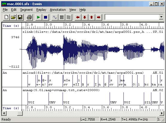
Figure 2.2 - Mapped annotations
Export of data to HTK format
Unfortunately, HTK cannot (as yet) read SFS files directly, so the next step is to export the data into files formatted so that HTK can read them. Fortunately, SFS knows how to read and write HTK formatted files. To write a set of HTK data files from the voc19 analysis we performed, just type:
$ apply "colist -H" ma*.sfs
This creates a set of HTK format data files with names modelled after the SFS files. Similarly to write a set of HTK format label files, use:
$ apply "anlist -h -O" ma*.sfs
We now have a set of data files ma*.dat and a set of label files ma*.lab in HTK format ready to train some HMMs.
HTK configuration
For training HMMs, HTK requires us to build some configuration files beforehand.
The first file is a general configuration of all HTK tools. We'll put this into a file
called config.txt
# config.txt - HTK basic parameters SOURCEFORMAT = HTK TARGETKIND = FBANK NATURALREADORDER = T |
In this file we specify that the source files are in HTK format, that the training data is already processed into filterbank parameters, and that the data is stored in the natural byte order for the machine.
The second configuration file we need is a prototype hidden Markov model which we will use to create the models for the three different labels. This configuration file is specific to a one-state HMM with a 19-dimensional observation vector, so we save it in a file called proto-1-19.hmm
<BeginHMM> <NumStates> 3 <VecSize> 19 <FBANK> <State> 2 <Mean> 19 0.0 0.0 0.0 0.0 0.0 0.0 0.0 0.0 0.0 0.0 0.0 0.0 0.0 0.0 0.0 0.0 0.0 0.0 0.0 <Variance> 19 1.0 1.0 1.0 1.0 1.0 1.0 1.0 1.0 1.0 1.0 1.0 1.0 1.0 1.0 1.0 1.0 1.0 1.0 1.0 <TransP> 3 0.0 1.0 0.0 0.0 0.9 0.1 0.0 0.0 1.0 <EndHMM> |
It is confusing that an HTK configuration file for a 1-state HMM has 3 states, but the HTK convention is that the first state and the last state are non-emitting, that is they are part of the nework of HMMs but do not describe any of the input data. Only the middle state of the three emits observation vectors. Briefly this HMM definition file sets up a model with a single state which holds the mean and variance of the 19 filterbank channel parameters. The transition probability matrix simply says that state 1 always jumps to state 2, that state 2 jumps to state 3 with a probability of 1 in 10, and that state 3 always jumps to itself.
HTK training
To train the HMMs we need a file containing a list of all the data files we will use for
training. Here we call it train.lst, and it has these contents:
mac.0002.dat mac.0003.dat mac.0004.dat mae.0001.dat mae.0003.dat mae.0004.dat maf.0001.dat maf.0002.dat maf.0004.dat mah.0001.dat mah.0002.dat mah.0003.dat |
We can now use the following script to train the HMMs:
# dotrain.sh
for s in SIL VOI UNV
do
    cp proto-1-19.hmm $s.hmm
    HRest -T 1 -C config.txt -S train.lst -l $s $s.hmm
done
|
In this script we copy our prototype HMM into SIL.hmm, VOI.hmm, UNV.hmm and then train these HMMs individually using the portions of the data files that are labelled with SIL, VOI and UNV respectively.
HTK testing
To evaluate how well our HMMs can label an unseen speech signal with the three labels, we recognise the data we reserved for testing and compare the recognised labels with the labels we generated. We'll show how to do the recognition in this section and look at performance evaluation in the next.
To recognise a data file using our trained HMMs we need three further HTK configuration files and a list of test files. The first configuration file we need is just a list of the HMMs, store this in a file called phone.lst:
SIL VOI UNV |
The next file we need is a dictionary that maps word pronunciations to a sequence of phone pronunciations. This sounds rather odd in this application, but is necessary because HTK is set up to recognise words rather than phones. Since we are really building a kind of phone recogniser, we solve the problem by having a dictionary of exactly three "words" each of which is "pronounced" by one of the phone labels. Put this into a file called phone.dic:
SIL SIL VOI VOI UNV UNV |
The last configuration file we need is a recognition grammar which describes which HMM sequences are allowed and what the probability is that each model should follow one of the others. For now, we will just use a default grammar consisting of a simple "phone loop" where the symbols can come in any order and with equal likelihood. This kind of grammar can be built using the HTK program HBuild from the phone list, as follows:
$ HBuild phone.lst phone.net
The resulting grammar file phone.net looks like this:
VERSION=1.0 N=7 L=9 I=0 W=!NULL I=1 W=!NULL I=2 W=SIL I=3 W=VOI I=4 W=UNV I=5 W=!NULL I=6 W=!NULL J=0 S=0 E=1 l=0.00 J=1 S=5 E=1 l=0.00 J=2 S=1 E=2 l=-1.10 J=3 S=1 E=3 l=-1.10 J=4 S=1 E=4 l=-1.10 J=5 S=2 E=5 l=0.00 J=6 S=3 E=5 l=0.00 J=7 S=4 E=5 l=0.00 J=8 S=5 E=6 l=0.00 |
Don't worry too much about this file. It looks more complex than it really is - basically the lines starting with "I" represent nodes of a simple transition network, while the lines starting with "J" represent arcs that run from one node to another and have a transition probability (stored as a log likelihood).
The last thing we need is a list of test filenames, put this in test.lst:
mac.0001.dat mae.0002.dat maf.0003.dat mah.0004.dat mam.0001.dat mam.0002.dat mam.0003.dat mam.0004.dat |
Recognition can be performed with the following script. We run HVite to generate a set of recognised label files (with a .rec file extension) then load them into the SFS files for evaluation:
# dotest.sh
HVite -T 1 -C config.txt -w phone.net -o S -S test.lst phone.dic phone.lst
for f in `cat test.lst`
do
    g=`echo $f | sed s/.dat//`
    anload -h $g.rec $g.sfs
done
|
In this script, the HVite option "-w phone.net" instructs it to perform word recognition, while the option "-o S" requests it not to put numeric scores in the recognised label files. The loop at the bottom takes the name of each test data file in turn, strips off the .dat from its name and loads the .rec file into the .sfs file with the SFS program anload.
Performance evaluation
We are now in a position to evaluate how well our system is able to divide a speech signal up into SIL-VOI-UNV. The input to the evaluation process are the SFS files for the test data. These now have the original acoustic annotations, the mapped annotations and the recognised annotations, see Figure 2.3.
Figure 2.3 - Recognition results
The figure shows that the recognised annotations are not bad, but there are some mistakes. We now need to consider what numerical measure we might use to describe the performance of the recogniser. In this case a suitable measure is the frame labelling rate: the percentage of frames of the signal which have been classified correctly. Since the recognised labels have been based on a frame rate of 100 frames per second, it also makes sense to evaluate the recognition performance at this rate.
The SFS program ancomp compares two annotation sets in various ways. It is supplied with a reference set and a test set and it can compare the timing of the labels, the content of the labels or the sequence of the labels. Here we want to look at the content of the labels every 10ms and build a confusion matrix that identifies which input (=reference) labels have been mapped to which output (=test) labels with what frequency. The command and some output for a single test file follows:
$ ancomp -r an.02 -t an.03 -f mac.0001.sfs
      SIL  UNV  VOI
SIL: 1114   31    6
UNV:   57  639  100
VOI:  140  138 1514
The "-f" switch to ancomp selects the frame labelling mode of comparison, while the switches "-r" and "-t" specify the reference and the test annotation items respectively. This way of running ancomp only delivers performance on a single file however, and we would like to get the performance over all test files. We can do this by asking ancomp to
dump its raw label comparisons to its output and then combine the outputs from the program across all test files. This output can then be sent to the SFS program conmat which is a general purpose program for producing confusion matrices. The script is as follows:
# doperf.sh
(for f in `cat test.lst`
do
    g=`echo $f|sed s/.dat//`
    ancomp -r an.02 -t an.03 -f -m - $g.sfs
done) | conmat -esl
|
If we run this on all the test files, we get this overall performance assessment:
$ sh doperf.sh
Processing date     : Mon Jun 28 12:44:05 2004
Confusion data from : stdin

    Confusion Matrix

     |  SIL   UNV   VOI
-----+-----------------
  SIL| 8130   855   151   9136 total  88%
  UNV|  888  5010  1631   7529 total  66%
  VOI|  736   863 12298  13897 total  88%

Number of matches = 30562
Recognition rate  =  83.2%
A way of diagnosing where the recognition is failing is to look at the mapping from the original acoustic annotations to the recognised SIL-VOI-UNV labels. We can do this for a single file as follows:
$ ancomp -r an.01 -t an.03 -f mac.0001.sfs
       SIL UNV VOI
    #:  12   1   0
   ##: 903   2   0
    +:  10   7   0
    /:   0   0   0
   3::   0   0  28
  3:?:   0   0   4
   =n:  15   6  25
  =nf:   0   0   1
    @:   1   6 144
   @?:   2   7  15
  @U@:   0   1  28
  @UU:   0   0  18
   @f:   0   8  11
   @~:   0   1  65
   A::   0   1  54
  A:f:   0   0   1
  A:~:   0   0   3
    D:  11   5  14
...
We could study this output to see whether we had made mistakes in our mapping from acoustic labels to classes.
Our little project could be extended in a number of ways:
- Use a different acoustic feature set. A popular spectral envelope feature set are mel-scaled cepstral coefficients (MFCCs). These can be calculated with the SFS program
mfcc. - Use a different HMM configuration. It is possible that a 3-state rather than 1-state HMM would perform better on this task, although care would have to be taken that it was still capable of recognising segments which were shorter than 3 spectral frames.
- Use a different density function. Since we are mapping a wide range of spectral vectors to a few classes, it is likely that the spectral density function for each class will not be normally distributed. The use of Gaussian mixtures within the HMMs may help.
- Use of full covariance. The 19 channels of the filterbank have a significant degree of covariation which may affect the accuracy of the probability estimates from the HMM. It may be better to use a full covariance matrix in the HMM rather than just a diagonal covariance.
- Use of symbol sequence constraints. Although unlikely to make much of an impact in this application, in many tasks there are constraints on the likely sequences of recognised symbols. HTK allows us to put estimated sequence probabilities in the recognition network.
3. Phone recognition
In this section we will build a simple phone recogniser. Again the aim is not to get ultimate performance, but to demonstrate the steps and the tools involved.
Source Data
Training a phone recogniser requires a lot of data. For a speaker dependent system you need several hundred sentences, while for a speaker-independent system you need several thousand. For this tutorial we will use the WSJCAM0 database. This is a database of British English recordings modelled after the Wall Street Journal database. The WSJCAM0 database is available from the Linguistic Data Consortium (www.ldc.upenn.edu). This database is large and comes with a phone labelling that makes it very easy to train a phone recogniser.
For the purposes of this tutorial we will just use a part of the speaker-independent training set. We will use speakers C02 to C0Z for training, and speakers C10 to C19 for testing. Within each speaker we only use the WSJ sentences, which are coded with a letter 'C' in the fourth character of the filename. The first thing to do is to obtain a list of file 'basenames' - just the directory name and basename of each file we will use for training and for testing. The following script will do the job:
# dogetnames.sh - get basenames of files for training and testing
rm -f basetrain.lst
for d in c:/data/wsjcam0/si_tr/C0*
do
  echo processing $d
  for f in $d/???C*.PHN
  do
    g=`echo $f | sed s/.PHN//`
    if test -e $g.WV1
    then
       h=`echo $g | sed s%c:/data/wsjcam0/si_tr/%%`
        echo $h >>basetrain.lst
    fi
  done
done
rm -f basetest.lst
for d in c:/data/wsjcam0/si_tr/C1[0-9]
do
  echo processing $d
  for f in $d/???C*.PHN
  do
    g=`echo $f | sed s/.PHN//`
    if test -e $g.WV1
    then
        h=`echo $g | sed s%c:/data/wsjcam0/si_tr/%%`
        echo $h >>basetest.lst
    fi
  done
done
|
The script looks for phonetic annotation files of the form "???C*.PHN" and as long as there is a matching audio signal ".WV1" it adds the basename of the file to a list. This script creates a file called "basetrain.lst" which has the speaker directory and base filename for each training file, and a file called "basetest.lst" which has the speaker directory and base filename for each test file. For the data used, there are about 3000 files in basetrain.lst and 900 in basetest.lst.
We can now load the audio signal and the source phonetic annotations into an SFS file using the following script:
# domakesfs.sh # # 1. make training and testing directories # mkdir train test for d in 2 3 4 5 6 7 8 9 A B C D E F G H I J K L M N O P Q R S T U V W X Y Z do mkdir train/C0$d done for d in 0 1 2 3 4 5 6 7 8 9 do mkdir test/C1$d done # # 2. convert audio and labels to SFS # for f in `cat basetrain.lst` do hed -n train/$f.sfs cnv2sfs c:/data/wsjcam0/si_tr/$f.wv1 train/$f.sfs anload -f 16000 -s c:/data/wsjcam0/si_tr/$f.phn train/$f.sfs done for f in `cat basetest.lst` do hed -n test/$f.sfs cnv2sfs c:/data/wsjcam0/si_tr/$f.wv1 test/$f.sfs anload -f 16000 -s c:/data/wsjcam0/si_tr/$f.phn test/$f.sfs done |
This script decompresses the audio signals in the ".WV1" files and loads in the phonetic annotations. The SFS files are created in "train" and "test" subdirectories of the tutorial folder:
$ mkdir tutorial2
$ cd tutorial2
$ sh dogetnames.sh
$ sh domakesfs.sh
Figure 3.1 shows an example source data file with an audio signal and phonetic annotations.
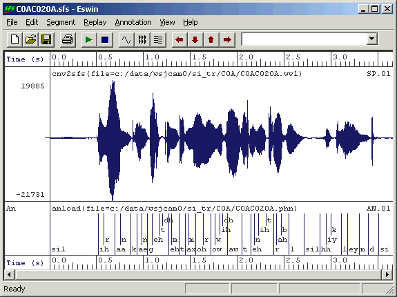
Figure 3.1 - Source data from WSJCAM0
Making HTK data files
We can now choose an acoustic feature set for the data and generate suitable HTK format data files and label files.
A very common type of acoustic feature set for phone recognition is based on mel-scaled cepstral coefficients (MFCCs). To keep things simple, we will use 12 MFCC parameters plus one parameter that is the log energy for each 10ms frame of signal. We will use the SFS program mfcc for this, but in fact HTK has its own tool for calculating MFCCs. Also for speed we will not use delta or delta-delta coefficients although these have been shown to improve recognition performance in some circumstances. The following shell script performs the MFCC calculation, saves the data into an HTK format file and records the HTK file names in 'train.lst' and 'test.lst' for us to use when we are training and testing HMMs.
# domakedat.sh # rm -f train.lst for f in `cat basetrain.lst` do mfcc -n12 -e -l100 -h6000 train/$f.sfs colist -H train/$f.sfs echo train/$f.dat >>train.lst done rm -f test.lst for f in `cat basetest.lst` do mfcc -n12 -e -l100 -h6000 test/$f.sfs colist -H test/$f.sfs echo test/$f.dat >>test.lst done |
To save producing one HTK label file per data file, we will create an HTK "Master Label File" which will hold all the phone labels for all files. Master label files can be built using the HTK HLEd program, but here we will use an SML script. This is easier to run and allows us to collect a list of the phone names and build a phone dictionary at the same time. The SML script is as follows:
/* makemlf.sml - make HTK MLF file from files */

/* table to hold annotation labels */
string    table[1:1000];
var    tcount;

/* MLF file */
file    op;

/* function to check/add label */
function var checklabel(str)
{
    string str;

    if (entry(str,table)) return(0);
    tcount=tcount+1;
    table[tcount]=str;
    return(1);
}

/*initialise */
init {
    openout(op,"phone.mlf");
    print#op "#!MLF!#\n";
}

/* for each input file */
main {
    var        i,num;
    string     basename;
    string    label;

    /* print filename */
    print $filename,"\n"
    i=index("\.",$filename);
    if (i) basename=$filename:1:i-1 else basename=$filename;
    print#op "\"",basename,".lab\"\n";

    /* print annotations */
    num=numberof(".");
    for (i=1;i<=num;i=i+1) {
        label = matchn(".",i);
        print#op label,"\n";
        checklabel(label);
    }
    print#op ".\n"
}

/* output phone list and dictionary */
summary {
    var    i,j;
    string    t;

    /* insertion sort */
    for (i=2;i<=tcount;i=i+1) {
        j=i;
        t=table[j];
        while (compare(t,table[j-1])<0) {
            table[j] = table[j-1];
            j=j-1;
            if (j==1) break;
        }
        table[j]=t;
    }

    /* close MLF file */
    close(op);

    /* write phone list */
    openout(op,"phone.lst");
    for (i=1;i<=tcount;i=i+1) print#op table[i],"\n";
    close(op);

    /* write phone+ list */
    openout(op,"phone+.lst");
    print#op "!ENTER\n";
    print#op "!EXIT\n";
    for (i=1;i<=tcount;i=i+1) print#op table[i],"\n";
    close(op);

    /* write phone dictionary */
    openout(op,"phone.dic");
    print#op "!ENTER []\n";
    print#op "!EXIT []\n";
    for (i=1;i<=tcount;i=i+1) print#op table[i],"\t",table[i],"\n";
    close(op);
}
|
This script is run as follows:
$ sml -f makemlf.sml train test
The "-f" switch to SML means that it ignores non SFS files when it searches directories and sub-directories for files. The output is "phone.mlf" - the HTK master label file, "phone.lst" - a list of the phone labels used in the data, "phone+.lst" - a list of the phones augmented with enter and exit labels, and "phone.dic" a dictionary in which phone "word" symbols are mapped to phone pronunciations (see section 2 for explanation!).
Training HMMs
To start we will need an HTK global configuration file just as we had in section 2. Here it is again - put this in "config.txt":
# config.txt - HTK basic parameters SOURCEFORMAT = HTK TARGETKIND = MFCC_E NATURALREADORDER = T |
We are now in a position to train a set of phone HMMs, one model per phone type. We'll construct these in a fairly conventional way with 3 states and no skips, with one gaussian mixture of 13 dimensions per state. Put the following in a file "proto-3-13.hmm":
<BeginHMM> <NumStates> 5 <VecSize> 13 <MFCC_E> <State> 2 <Mean> 13 0.0 0.0 0.0 0.0 0.0 0.0 0.0 0.0 0.0 0.0 0.0 0.0 0.0 <Variance> 13 1.0 1.0 1.0 1.0 1.0 1.0 1.0 1.0 1.0 1.0 1.0 1.0 1.0 <State> 3 <Mean> 13 0.0 0.0 0.0 0.0 0.0 0.0 0.0 0.0 0.0 0.0 0.0 0.0 0.0 <Variance> 13 1.0 1.0 1.0 1.0 1.0 1.0 1.0 1.0 1.0 1.0 1.0 1.0 1.0 <State> 4 <Mean> 13 0.0 0.0 0.0 0.0 0.0 0.0 0.0 0.0 0.0 0.0 0.0 0.0 0.0 <Variance> 13 1.0 1.0 1.0 1.0 1.0 1.0 1.0 1.0 1.0 1.0 1.0 1.0 1.0 <TransP> 5 0.0 1.0 0.0 0.0 0.0 0.0 0.6 0.4 0.0 0.0 0.0 0.0 0.6 0.4 0.0 0.0 0.0 0.0 0.7 0.3 0.0 0.0 0.0 0.0 1.0 <EndHMM> |
We now initialise this model to be "flat" - that is with each state mean set to the global data mean and each state variance set to the global data variance. The HTK tool HCompV will do this, as follows:
$ HCompV -T 1 -C config.txt -m -S train.lst -o proto.hmm proto-3-13.hmm
This creates a file "proto.hmm" with the <MEAN> and <VARIANCE> sections initialised to appropriate values. We now need to duplicate this prototype into a model for each phone symbol type. We can do this with a shell script as follows:
# domakehmm.sh
HCompV -T 1 -C config.txt -m -S train.lst -o proto.hmm proto-3-13.hmm
head -3 proto.hmm > hmmdefs
for s in `cat phone.lst`
do
  echo "~h \"$s\"" >>hmmdefs
  gawk '/BEGINHMM/,/ENDHMM/ { print $0 }' proto.hmm >>hmmdefs
done
|
Run this script to creates a file "hmmdefs" which has a model entry for each phone all initialised to the same mean values.
We can now train the phone models using the HTK embedded re-estimation tool HERest.
The basic command is as follows:
$ HERest -C config.txt -I phone.mlf -S train.lst -H hmmdefs phone.lst
This command re-estimates the HMM parameters in the file hmmdefs, returning the updated model to the same file. This command needs to be run several times, as the re-estimation process is iterative. To decide how many cycles of re-estimation to perform it is usual to monitor the performance of the recogniser as it trains and to stop training when performance peaks. For this to work we need to test the recogniser on material that hasn't been used for training, and for honesty won't be used for the final performance evaluation either.
To estimate the performance of the recogniser, we use it to recognise our reserved test data and compare the recognised transcriptions to the ones distributed with the database. To perform recognition we need the phone.lst file which lists the names of the models, the phone.dic file which maps the phone names onto themselves, and a phone.net file which contains the recognition grammar. In this application it makes sense to use a bigram grammar in which we record the probabilities that one phone can follow another. We can build this with the commands:
$ HLStats -T 1 -C config.txt -b phone.big -o phone.lst phone.mlf
$ HBuild -T 1 -C config.txt -n phone.big phone+.lst phone.net
The HLStats command collects bigram statistics from our master label file and stores them in phone.big. The HBuild command converts these into a network grammar suitable for recognition. The phone+.lst file is the list of phone models augmented with the symbols "!ENTER" and "!EXIT".
The basic recognition command, now, is just:
$ HVite -T 1 -C config.txt -H hmmdefs -S test.lst -i recout.mlf \
-w phone.net phone.dic phone.lst
This command runs the recogniser and stores its recognition output in the recout.mlf master label file. To compare the recognised labels to the distributed labels, we can use the HResults program:
$ HResults -I phone.mlf phone.lst recout.mlf
====================== HTK Results Analysis =======================
  Date: Thu Jul  1 09:10:58 2004
  Ref : phone.mlf
  Rec : recout.mlf
------------------------ Overall Results --------------------------
SENT: %Correct=0.00 [H=0, S=903, N=903]
WORD: %Corr=48.03, Acc=41.52 [H=31884, D=10898, S=23605, I=4319, N=66387]
===================================================================
We can put this all together in a script which runs through 10 cycles of re-estimation and collects the performance after each cycle in a log file:
# dotrainrec.sh rm -f log for n in 1 2 3 4 5 6 7 8 9 10 do HERest -T 1 -C config.txt -I phone.mlf -S train.lst -H hmmdefs phone.lst HVite -T 1 -C config.txt -H hmmdefs -S test.lst -i recout.mlf \ -w phone.net phone.dic phone.lst echo "Cycle $n:" >>log HResults -I phone.mlf phone.lst recout.mlf >>log done |
Figure 3.2 shows how the Accuracy figure changes with training cycle on our data:
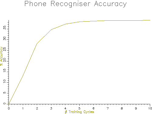
Figure 3.2 - Phone recognition accuracy with number of training cycles
Our recogniser seems to reach a maximum performance of about 40% phone accuracy. This is not very good, the best phone recognisers on this data have an accuracy of 70%.
Parameter Analysis
One possible contributory factor to the relatively poor performance of our phone recogniser might be the use of single gaussian (normal) distributions for the modelling of the cepstral coefficient variation within a state. We can easily write an SML script to investigate whether the actual distributions are not modeled well by a gaussian distribution. The following script asks for a segment label and then scans the source SFS files to build histograms of the first 12 cepstral coefficients as they vary within instances of that segment. The distributions are plotted with an overlay of a normal distribution.
/* codist.sml - plot distributions of MFCC data values */

/* raw data */
var    rdata[12,100000];
var    rcount;

/* distributions */
stat    rst[12];

/* segment label to analyse */
string    label;

/* graphics output */
file gop;

/* normal distribution */
function var normal(st,x)
stat st;
{
    var x;
    x = x - st.mean;
    return(exp(-0.5*x*x/st.variance)/sqrt(2*3.14159*st.variance));
}

/* plot histogram overlaid with normal distribution */
function var plotdist(gno,st,tab,tcnt)
stat st;
var tab[];
{
    var gno;
    var tcnt;
    var i,j,nbins,bsize;
    var hist[0:100];
    var xdata[1:2];
    var ydata[0:10000];

    /* find maximum and minimum in table */
    xdata[1]=tab[gno,1];
    xdata[2]=tab[gno,1];
    for (i=2;i<=tcnt;i=i+1) {
        if (tab[gno,i] < xdata[1]) xdata[1]=tab[gno,i];
        if (tab[gno,i] > xdata[2]) xdata[2]=tab[gno,i];
    }

    /* set up x-axes */
    plotxdata(xdata,1)

    /* estimate bin size */
    nbins = sqrt(tcnt);
    if (nbins > 100) nbins=100;
    bsize = (xdata[2]-xdata[1])/nbins;

    /* calculate histogram */
    for (i=1;i<=tcnt;i=i+1) {
        j=trunc((tab[gno,i]-xdata[1])/bsize);
        hist[j]=hist[j]+1/tcnt;
    }

    /* plot histogram */
    plotparam("title=C"++istr(gno));
    plotparam("type=hist");
    plot(gop,gno,hist,nbins);

    /* plot normal distribution */
    plotparam("type=line");
    for (i=0;i<=10*nbins;i=i+1) ydata[i]=bsize*normal(st,(xdata[1]+i*bsize/10));
    plot(gop,gno,ydata,10*nbins);
}

/* get segment name */
init {
    print#stderr "For segment : ";
    input label;
}

/* for each input file */
main {
    var i,j,num
    var    t,et;

    if (rcount >= 100000) break;

    num=numberof(label);
    for (i=1;i<=num;i=i+1) {
        t = next(CO,timen(label,i));
        et = t + lengthn(label,i);
        while (t < et) {
            if (rcount >= 100000) break;
            rcount=rcount+1;
            for (j=1;j<=12;j=j+1) {
                rdata[j,rcount] = co(4+j,t);
                rst[j] += co(4+j,t);
            }
            t = next(CO,t);
        }
    }
}

/* plot */
summary {
    var j;

    openout(gop,"|dig -g -s 500x375 -o dig.gif");
    plottitle(gop,"MFCC Distributions for /"++label++"/");
    plotparam("horizontal=4");
    plotparam("vertical=3");

    for (j=1;j<=12;j=j+1) plotdist(j,rst[j],rdata,rcount);
}
|
This script can be run as
$ sml -f codist.sml train
For segment : r
Two outputs of the script are shown in Figures 3.3 and 3.4.
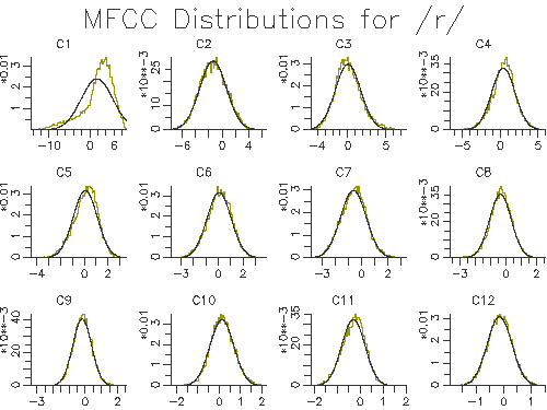
Figure 3.3 - Modelled cepstral distributions for /r/
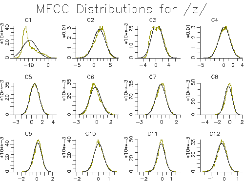
Figure 3.4 - Modelled cepstral distributions for /z/
The figures show that a single gaussian distribution is quite good for most of the cepstral coefficients, but not for the first cepstral coefficient. This implies that we may get a small performance improvement by changing to more than one gaussian per state. To increase the number of gaussian mixtures on all phone models (for all cepstral coefficients) we can use the HTK program HHed. This program is a general purpose HMM editor and takes as input a control file of commands. In this case we just want to increase the number of mixtures on all states. Put this in a file called mix2.hed:
MU 2 {*.state[2-4].mix}
|
Then the HMMs can be edited with the command
$ HHed -H hmmdefs mix2.hed phone.lst
A few more cycles of training can now be applied to see the effect.
Viewing recognition results in SFS
The output of the phone recogniser above is an HTK master label file recout.mlf.
If we want to view these results within SFS we need to load these as annotations. We can do this directly with the SFS program anload. First we take a copy of a test file, then
load in the annotations corresponding to that file from the master label file:
$ cp test/c10/c10c020v.sfs .
$ anload -H recout.mlf test/c10/c10c020v.rec c10c020v.sfs
$ eswin -isp -aan c10c020v.sfs
Notice that the anload program takes the name of the MLF file and the name of the section in the file to load. The SFS program eswin displays the speech and annotations in the file, as shown in Figure 3.5.
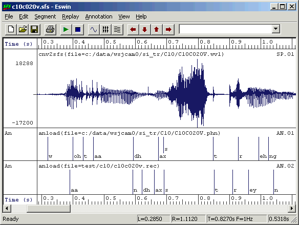
Figure 3.5 - Viewing recognition results
Although the HTK program HResults can analyse the performance of our recogniser on the test data and the confusions it makes, we can also perform a similar analysis in SFS for single or multiple files. The process is to load the recognised phone labels into SFS and then use the ancomp program in its "labelling" mode. We can do this on a single file with:
$ cp test/c10/c10c020v.sfs .
$ anload -H recout.mlf test/c10/c10c020v.rec c10c020v.sfs
$ ancomp -l c10c020v.sfs
Subst=21 Delete=6 Insert=5 Total=64 Accuracy=59.4%
To compare multiple files, we get ancomp to list its raw phone alignments to a file and then input the collected output to the confusion matrix program. Here is a script to do this:
# doancomp.sh
#
# collect mappings
(for f in `cat basetest.lst`
do
    cp test/$f.sfs temp.sfs
    anload -H recout.mlf test/$f.rec temp.sfs
    ancomp -l -m - temp.sfs
done) >ancomp.lst
rm temp.sfs
#
# build confusion matrix
conmat -esl ancomp.lst >conmat.lst
|
The file conmat.lst contains a large phoneme confusion matrix as well as an overall performance score. Since this is rather unwieldy, it is also interesting just to find the most common confusions. We can generate a list of confusions from ancomp.lst using some unix trickery:
$ gawk '{ if ( $1 != $2 ) print $0 }' ancomp.lst | sort | uniq -c | \
  sort -rn | head -20
    882 [] sil
    820 ax []
    724 t []
    616 ih []
    468 ih ax
    415 n m
    409 ih iy
    373 ih uw
    373 d []
    367 n []
    325 s z
    313 l []
    289 r []
    283 t s
    278 n ng
    268 dh []
    266 [] d
    264 l ao
    262 ax ih
    262 ax ah
The most common confusions are probably what we would expect: insertions of silence, deletions of /@/, /t/ and /I/, substitutions of /I/ with /@/, or /m/ for /n/, and so on. How this command works is left as an exercise for the reader!
Enhancements
We might improve the performance of the phone recogniser in a number of ways:
- Add delta coefficients: adding the rate of change of each acoustic parameter to the feature set (deltas) has been shown to improve phone recognition, performance as has the addition of accelerations (delta-deltas). You can do this easily by changing the type of the HMM to
MFCC_E_D_A. - Build phone in context models: building phone models which are different according to the context in which they occur can help a great deal. A typical approach to this is to build "triphone" models - where we build a model for each phone for every pair of possuble left and right phones in the label files. Since this requires more data than we have typically, it is also necessary to smooth the probability estimates araising from training by "state-tying" - using the data over many triphone contexts to estimate observations for a state of one triphone model. This procedure is usually performed in a data-driven way using clustering methods. The HTK documentation gives details.
- Add a phone language model: although our recogniser uses bigram probabilities to constrain recognition, there are also useful constraints on sequences longer than two phones that would help recognition. HTK does not have a simple way of doing this, but one might expect that 3-gram, 4-gram or even 5-gram phone grammars would help considerably.
4. Word recognition
Once we have built a phone recogniser, it is a simple matter to extend it to recognise words. Of course it is also possible to build a word recogniser in which each word is modelled separately with an HMM.
Dictionary
To build a word recogniser from a phone recogniser, we first need a dictionary that maps words to phone sequences. Here is an example for a simple application. Put this in digits.dic:
ZERO z ia r ow ZERO ow ONE w ah n TWO t uw THREE th r iy FOUR f ao FOUR f ao r FIVE f ay v SIX s ih k s SEVEN s eh v n EIGHT ey t NINE n ay n WHAT-IS w oh t ih z PLUS p l ah s MINUS m ay n ax s TIMES t ay m z DIVIDED-BY d ih v ay d ih d b ay SIL [] sil |
Grammar
Next we need a grammar file which constrains the allowed word order. The more constraints we can put here, the more accurate our recogniser. Here is a simple grammar file that allows us to recognise phrases such as "what is two plus five". Put this in digits.grm:
$digit = ONE | TWO | THREE | FOUR | FIVE | SIX | SEVEN | EIGHT | NINE | ZERO; $operation = PLUS | MINUS | TIMES | DIVIDED-BY; ( SIL WHAT-IS <$digit> $operation <$digit> SIL ) |
To convert this file to a form that the recogniser can use, we need to run the HTK tool HParse, as follows:
$ HParse digits.grm digits.net
Word recogniser
The basic command for recognising HTK data file inp.dat using our digits task recogniser is then just:
$ HVite -T 1 -C config.txt -H hmmdefs -w digits.net digits.dic \
  phone.lst inp.dat
We can put together a simple script that uses SFS to acquire an audio signal, then performs an MFCC analysis, exports the coefficients to HTK and runs the recogniser:
# doreclive.sh
rm -f inp.sfs
hed -n inp.sfs >/dev/null
echo "To STOP this script, type CTRL/C"
#
remove -e inp.sfs >NUL
echo "***** Say Word *****"
while record -q -e -f 16000 inp.sfs
do
  replay inp.sfs
  mfcc -n12 -e -l100 -h6000 inp.sfs
  colist -H inp.sfs
  HVite -T 1 -C config.txt -H hmmdefs -w digits.net digits.dic \
    phone.lst inp.dat
  remove -e inp.sfs >NUL
  echo "***** Say Word *****"
done
|
You could also use the HTK live audio input facility for this demonstration. But then you should also use the HTK MFCC analysis in training as well, as the HTK MFCC analysis gives slightly different scaled coefficient values than the SFS program mfcc.
Enhancement
We might enhance our word recogniser in a number of ways:
- Use a better set of phone models, for example with triphones
- For a small vocabulary and lots of training data, it is better to build word-level models.
- For a large vocabulary it is better to use a statistical language model, such as a trigram model rather than trying to build a grammar.
- Model non-speech regions and silent gaps more intelligently, by having models for noises and inter-word silent gaps for example.
5. Phone alignment
Another application for our phone recogniser is phone alignment. In phone alignment we have an unlabelled audio signal and a transcription and the task is to align the transcription to the signal. This procedure is already implemented as part of SFS using the program analign, but we will show the basic operation of analign here.
Assume we have an audio recording of a single sentence, here it is the sentence "six plus three equals nine" stored in an sfs file called six.sfs. We first perform MFCC analysis on the audio signal:
$ mfcc -n12 -e -l100 -h6000 six.sfs
We next add an annotation containing the raw transcription in ARPABET format:
$ anload -t phone -T "sil s ih k s p l ah s th r iy iy k w ax l z n ay n sil" six.sfs
Then export both coefficients and annotations to HTK format:
$ colist -H six.sfs
$ anlist -h -O six.sfs
We can now run the HTK HVite program in alignment mode with:
$ HVite -C config.txt -a -o SM -H hmmdefs phone.dic phone.lst six.dat
And load the aligned annotations back into SFS:
$ anload -h six.rec six.sfs
The result is shown in figure 5.1.
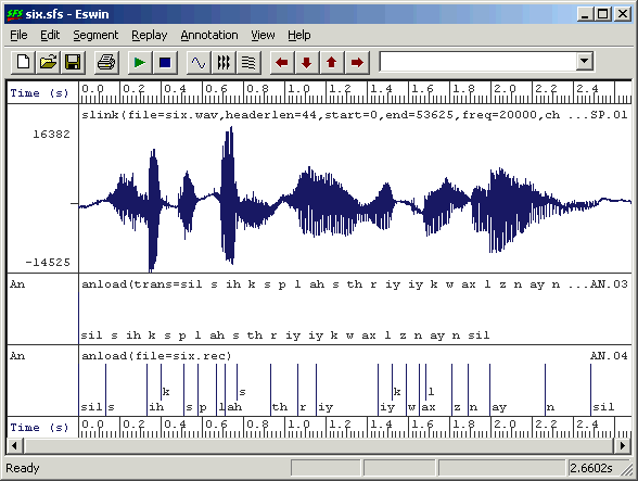
Figure 5.1 - Aligned phone labels
The SFS program analign makes this process easier by handling all the export and import of data to HTK and also handles the chopping of large files into sentence sizes pieces and the translation of symbol sets between SAMPA, ARPABET and JSRU.
6. Pronunciation variation analysis
A variation on phone alignment is to provide a shallow network of pronunciation alternatives to HVite and let it choose which pronunciation was actually used by a speaker. This kind of variation analysis could be useful in the study of accent variation.
In this example, we will take a sentence spoken by two different speakers of two different regional accents of the British Isles. The sentence is "after tea father fed the cat", and we are interested whether the vowel /{/ or /A:/ was used in the words "after" and "father". For reference, we always expect "cat" to be produced with /{/, so we will check on the analysis by also looking to see if the program rejects the pronunciation of "cat" as /kA:t/.
We first create a dictionary file the sentence. Put this in accents.dic:
AFTER aa f t ax AFTER ae f t ax TEA t iy FATHER f aa dh ax FATHER f ae dh ax FED f eh d THE dh ax CAT k aa t CAT k ae t SIL [] sil |
Notice that the dictionary lists the alternative pronunciations that we are interested in. Next we create a grammar just for this sentence. Put this in accents.grm
( SIL AFTER TEA FATHER FED THE CAT SIL ) |
Next we convert the grammar file to a recognition network with HParse:
$ HParse accents.grm accents.net
Then we prepare HTK data files for the two audio signals:
$ mfcc -n12 -e -l100 -h6000 brm.sfs
$ mfcc -n12 -e -l100 -h6000 sse.sfs
$ colist -H brm.sfs
$ colist -H sse.sfs
Then we recognise the utterances using the grammar, but outputting the selected phone transcription.
$ HVite -C config.txt -H hmmdefs -w accents.net -m -o ST accents.dic \
  phone.lst brm.dat sse.dat
The "-m" switch to HVite causes the phone model names to be output to the recognised label files, while the "-o ST" switch cause the scores and the times to be suppressed.
The output of the recogniser are in brm.rec and sse.rec as follows:
brm.rec | sse.rec | |
|---|---|---|
sil SIL ae AFTER f t ax t TEA iy f FATHER aa dh ax f FED eh d dh THE ax k CAT ae t sil SIL |
sil SIL aa AFTER f t ax t TEA iy f FATHER aa dh ax f FED eh d dh THE ax k CAT ae t sil SIL |
From this it is easy to see that the Birmingham speaker used /{/ where the South-East speaker used /A:/ in "after".
7. Dysfluency recognition
Another application of phone recognition is the detection of dysfluencies. Although our phone recogniser is not particularly accurate we can still look for pattern in the recognised phone sequence which may be indicators of dysfluency. We will recognise a passage with the phone recogniser, load the phone labels into the SFS file then use an SML script to look for dysfluent patterns.
Here are the commands for performing MFCC analysis on the passage, saving the coefficients to HTK format, building a simple phone loop recogniser without bigram constraints, then running the recogniser and loading the phone annotations back into the file:
$ mfcc -n12 -e -l 100 -h 6000 dysfluent.sfs
$ colist -H dysfluent.sfs
$ HBuild phone.lst phone.net
$ HVite -C config.txt -H hmmdefs -w phone.net -o S phone.dic phone.lst dysfluent.dat
$ anload -h dysfluent.rec dysfluent.sfs
The following SML script takes the recognised phone sequence and looks for (i) single (non-silent) phones lasting for longer than 0.25s, (ii) repeated (non-silent) phone labels which together last for longer than 0.25s, (iii) patterns of five phone labels matching A-B-A-B-A where A is not silence. Output is another annotation item with the dysfluent regions marked with "(D)".
/* dysfind.sml - find dysfluencies from phone recogniser output */

/* input and output annotation sets */
item    ian;
item    oan;

/* table to hold dysfluent events */
var    times[1000,2];
var    tcount;

/* add times of dysfluencies to table */
function var addtime(posn,size)
{
    var posn,size;
    var i;

    /* put event in sorted position */
    i=tcount+1;
    if (i > 1) {
        while (posn < times[i-1,1]) {
            times[i,1] = times[i-1,1];
            times[i,2] = times[i-1,2];
            i = i - 1;
            if (i==1) break;
        }
    }
    times[i,1]=posn;
    times[i,2]=size;
    tcount=tcount+1;
}

/* check for continuant */
function var iscontinuant(label)
{
    string label;

    if (compare(label,"sil")==0) return(0);
    if (index("^[ptkpbg]$",label)) return(0);
    if (compare(label,"j")==0) return(0);
    if (compare(label,"ch")==0) return(0);
    return(1);
}

/* process each input file */
main {
    var    i,numf,fdur,dmin;
    var ocnt,size;
    string lab1,lab2,lab3;

    /* get input & output */
    sfsgetitem(ian,$filename,str(selectitem(AN),4,2));
    numf=sfsgetparam(ian,"numframes");
    fdur=sfsgetparam(ian,"frameduration");
    sfsnewitem(oan,AN,fdur,sfsgetparam(ian,"offset"),1,numf);

    /* put minimum dysfluency length = 0.33s */
    dmin = 0.33/fdur;

    /* look for long continuant annotations */
    tcount=0;
    for (i=1;i<=numf;i=i+1) {
        size = sfsgetfield(ian,i,1);
        if (size > dmin) {
            lab1 = sfsgetstring(ian,i);
            if (iscontinuant(lab1)==1) {
                addtime(sfsgetfield(ian,i,0),size);
            }
        }
    }

    /* look for patterns like AA */
    for (i=2;i<=numf;i=i+1) {
        lab1 = sfsgetstring(ian,i-1);
        lab2 = sfsgetstring(ian,i);
        if (compare(lab1,lab2)==0) {
            size = sfsgetfield(ian,i-1,1)+sfsgetfield(ian,i,1);
            if (size > dmin) {
                if (iscontinuant(lab1)==1) {
                    addtime(sfsgetfield(ian,i-1,0),size);
                }
            }
        }
    }

    /* look for patterns like AAA */
    for (i=3;i<=numf;i=i+1) {
        lab1 = sfsgetstring(ian,i-2);
        lab2 = sfsgetstring(ian,i-1);
        if (compare(lab1,lab2)==0) {
            lab3 = sfsgetstring(ian,i);
            if (compare(lab1,lab3)==0) {
                size = sfsgetfield(ian,i-2,1)+sfsgetfield(ian,i-1,1)+sfsgetfield(ian,i,1);
                if (size > dmin) {
                    if (iscontinuant(lab1)==1) {
                        addtime(sfsgetfield(ian,i,0),size);
                    }
                }
            }
        }
    }

    /* look for patterns like ABABA */
    for (i=5;i<=numf;i=i+1) {
        lab1 = sfsgetstring(ian,i-4);
        lab2 = sfsgetstring(ian,i-2);
        if ((compare(lab1,lab2)==0)&&(compare(lab1,"sil")!=0)) {
            lab3 = sfsgetstring(ian,i);
            if (compare(lab1,lab3)==0) {
                lab1 = sfsgetstring(ian,i-3);
                lab2 = sfsgetstring(ian,i-1);
                if (compare(lab1,lab2)==0) {
                    size = sfsgetfield(ian,i,0)+sfsgetfield(ian,i,1)-sfsgetfield(ian,i-4,0);
                    addtime(sfsgetfield(ian,i-4,0),size);
                }
            }
        }
    }

    /* convert times to annotations (ignoring overlaps) */
    ocnt=0;
    for (i=1;i<=tcount;i=i+1) {
        sfssetfield(oan,ocnt,0,times[i,1]);
        sfssetfield(oan,ocnt,1,times[i,2]);
        sfssetstring(oan,ocnt,"(D)");
        ocnt=ocnt+1;
        if ((i==tcount)||(times[i+1,1]>times[i,1]+times[i,2])) {
            sfssetfield(oan,ocnt,0,times[i,1]+times[i,2]);
            sfssetfield(oan,ocnt,1,times[i+1,1]-times[i,1]-times[i,2]);
            sfssetstring(oan,ocnt,"/");
            ocnt=ocnt+1;
        }
    }

    /* save output back to file */
    sfsputitem(oan,$filename,ocnt);
}
|
This script would be run with:
$ sml -ian^anload dysfind.sml dysfluent.sfs
Figure 7.1 shows one particular pattern of "ih sil ih sil ih" which is a real dysfluency detected by the script.
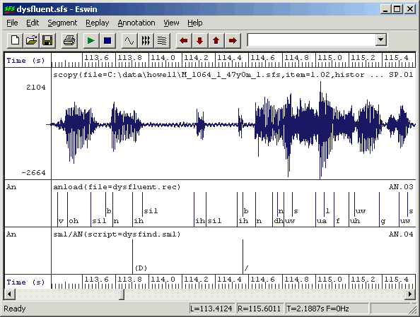
Figure 7.1 - Dysfluency recognition
To check the performance of the recogniser, we can compare the output of 'dysfind.sml' with some manual dysfluency annotations. In this example, the manual annotations contain the symbol "(D)" wherever there is a noticeable dysfluency. In this script we load the times of the manually marked dysfluencies and then compare them with the output of the recogniser and script. We get a "hit" if a manual and a recognised annotation overlap in time.
/* dysmark.sml - mark performance of dysfluency recogniser */

var mtab[1000,3];        /* time of each reference event */
var mcnt                /* number of reference events */
var nhit,nmiss,nfa        /* # hits, misses, false alarms */
var rtotal;                /* total reference events */
var ttotal;                /* total recognised events */

/* compare a recognised event to reference table */
function var markevent(t1,t2)
{
    var    t1,t2
    var    i

    for (i=1;i<=mcnt;i=i+1) {
        /* check for any overlap in time */
        if ((mtab[i,1]<=t1)&&(t1*lt;=mtab[i,2])) {
            nhit=nhit+1;
            mtab[i,3]=1;
            return(1);
        }
        if ((mtab[i,1]<=t2)&&(t2<=mtab[i,2])) {
            nhit=nhit+1;
            mtab[i,3]=1;
            return(1);
        }
    }
    /* must be a false alarm */
    nfa=nfa+1;
    return(0);
}

main {
    string    match
    var i,num
    var    t1,t2;

    /* load reference annotations into table */
    selectmatch("an^*fluency*word");
    match="^.*\(.*\).*$";
    num=numberof(match);
    for (i=1;i<=num;i=i+1) {
        mtab[i,1] = timen(match,i);
        mtab[i,2] = mtab[i,1] + lengthn(match,i);
        mtab[i,3] = 0;
    }
    mcnt=num;

    /* compare to recognised annotations */
    selectmatch("an^*dysfind");
    num=numberof("\(D\)");
    for (i=1;i<=num;i=i+1) {
        t1=timen("\(D\)",i);
        t2=t1+lengthn("\(D\)",i);
        markevent(t1,t2);
    }

    /* count misses */
    for (i=1;i<=mcnt;i=i+1) if (mtab[i,3]==0) nmiss=nmiss+1;

    /* update totals */
    rtotal = rtotal + mcnt;
    ttotal = ttotal + num;
}

summary {
    print "Total reference    = ",rtotal:1,"\n";
    print "Total recognised   = ",ttotal:1,"\n";
    print "Total hits         = ",nhit:1,"\n";
    print "Total misses       = ",nmiss:1,"\n";
    print "Total false alarms = ",nfa:1,"\n";
}
|
This script shows that we still have some way to go:
$ sml dysmark.sml dysfluent.sfs
Total reference    = 36
Total recognised   = 12
Total hits         = 2
Total misses       = 34
Total false alarms = 10
Bibliography
- BEEP British English pronunciation dictionary at
ftp://svr-ftp.eng.cam.ac.uk/pub/comp.speech/dictionaries/beep.tar.gz. - Hidden Markov modelling toolkit at http://htk.eng.cam.ac.uk/.
- International Phonetic Alphabet at http://www.arts.gla.ac.uk/IPA/ipachart.html.
- SAMPA Phonetic Alphabet at http://www.phon.ucl.ac.uk/home/sampa/.
- Speech Filing System at http://www.phon.ucl.ac.uk/resource/sfs/.
- SCRIBE corpus at www.phon.ucl.ac.uk/resource/scribe.
Feedback
Please report errors in this tutorial to sfs@pals.ucl.ac.uk. Questions about the use of SFS can be posted to the SFS speech-tools mailing list.