Department of Phonetics and Linguistics

AUDITORY FILTER NONLINEARITY AT 2kHz IN NORMAL AND IMPAIRED HEARING

Stuart ROSEN, Richard J. BAKER and Angela DARLING

The hearing-impaired listener with a greater loss (30 dB HL at 2 kHz) showed quite a different pattern of results. Her auditory filter shapes changed little with level. Filtering on the upper side of the filter was essentially normal, while that on the lower side could only be considered normal at relatively high levels. For low measurement levels, her auditory filter slopes were considerably shallower than normal on the low frequency side. The hearing-impaired listener with less loss (20 dB HL at 2 kHz) showed a degree of nonlinearity intermediate between this and the normal listeners. Thus, at least in these cases, hearing loss appears to consist of a loss of nonlinearity in the auditory periphery, leading to threshold elevation, loss of frequency selectivity at low levels, but no degradation of selectivity at relatively high levels. Physiological evidence suggests that this most likely arises from damage to the outer hair cells.

1. Introduction
A fundamental property of the peripheral auditory system is that it operates as a frequency analyser. This processing mechanism can be conceptualised as a bank of overlapping bandpass filters, often referred to as auditory filters. Some of the applications exploiting the concept of auditory filters (and requiring accurate auditory filter shape characterisation) include the design of realistic front ends for automatic speech recognition (Zwicker, Terhardt, & Paulus, 1979) and modelling the effects of normal and impaired cochlear tuning on the perception of speech or music (Patterson, Nimmo-Smith, Weber, & Milroy, 1982; Rosen & Fourcin, 1986). It has also been suggested that auditory filter shape measurement may be a useful diagnostic tool in the detection of preclinical noise-induced hearing loss (West & Evans, 1990).

The most well-developed psychoacoustic technique for measuring auditory filter shapes is the notched-noise simultaneous masking method, supported by an explicit analysis algorithm (for a review, see Patterson & Moore, 1986). Typically, thresholds are found for a tonal signal at a particular frequency in the presence of fixed-level band-stop noises (notched noises), with the varying-width notch placed both symmetrically and asymmetrically around the probe. The dependence of probe threshold on the notch configuration is exploited to estimate the auditory filter shape. Of course, we could also fix the level of the probe, and vary the masker level for a particular notch. Were auditory filters linear, it would not matter which level was fixed and which was varied. But it is now well known that auditory filters are highly nonlinear, broadening with increasing level. Therefore, it is crucial to decide whether to fix probe or masker level in such experiments. At a more fundamental level, we need to determine what it is about the stimulus configuration that controls the filter shape. If filter shapes are somehow controlled by probe level, then fixing the masker will distort considerably the shape of the imputed auditory filters, and vice versa.

It is perhaps surprising, then, that such a crucial issue has received relatively little attention until recently. Although two previous studies have claimed to decide this issue (Lutfi & Patterson, 1984; Moore & Glasberg, 1987), we have recently shown that such claims cannot be upheld (Rosen & Baker, 1994). Instead, we have developed quite a different approach, which is to explicitly model the changes in filter parameters as a function of level, and to determine whether a dependence of these parameters on masker level or probe level better accounts for the data.

To illustrate this idea in a relatively simple case, consider a notched-noise masking experiment performed with symmetric notches only, at a fixed masker level of N₀ dB SPL/Hz. Let us assume the symmetric roex(p,w,t) filter shape to be appropriate (Patterson et al., 1982):

In this way, it is possible to construct a single model which, after appropriate coefficients are chosen, can predict thresholds for any combination of notch widths and level. Fitting the model to the data proceeds in essentially the same way as for the single level case. Instead of searching the space of the parameter values directly for the best-fitting values, the space of the coefficients making up the polynomials is searched. Note that this fitting technique is quite different to the typical procedure used for studies across level, in which filter parameters are estimated separately for each of a number of masker levels, and polynomial fits are made to the values of the estimated parameters as a function of level. We have, for example, fit as many as 158 mean data points in a single analysis, instead of doing 10 separate analyses (5 conditions in which the probe level is fixed, and 5 in which the masker level is fixed). Thus, data from the fixed-probe and fixed-masker experiments can be analysed together, putting stronger constraints on the way filter parameters can change with level.

A primary advantage of the PolyFit procedure is one of stability of the model fit, because such a large number of conditions can be fit by relatively few free coefficients. For example, in fitting one set of fixed-masker data (involving 13-16 data points) with a roex(p,w,t) filter shape in which p, w and t are independently estimated on the upper and lower frequency side, 7 free parameters must be estimated (including k). To describe the filter shape as a function of level requires multiplying the number of parameters by, for example, 5 levels of N₀ and 5 levels of P_s (70 parameters for 160 data points). Using PolyFit to fit the same data with a roex(p,w,t) model in which each of the 7 parameters is allowed to take on the form of a linear function of N₀ (or P_s) results in a model with 14 coefficients (7 x 2) for the same number of data points. This large reduction in the number of free variables allows the stable fitting of complex models such as the roex(p,w,t) shape, something which was not possible using the 'standard' techniques (Patterson et al., 1982). PolyFit also provides a principled way of comparing data across fixed-masker and fixed-probe conditions. Individual fits leave these results incommensurable.

One further extension to typical roex fitting procedures was implemented. Because absolute thresholds can place a lower limit on masked thresholds in some conditions (for fixed noise maskers at low levels with wide notches), a single estimated parameter corresponding to the absolute threshold of the probe was incorporated. This was done by adding the value of the estimated threshold (in power terms) to the probe level predicted by the model for any particular condition. For probe levels more than 10 dB and 20 dB above the estimated absolute threshold, this term changes the initially predicted value by less than 0.5 dB and 0.05 dB, respectively.

Rosen and Baker (1994) report an application of PolyFit using a roex(p,r) shape to a set of data obtained from 2 normal-hearing listeners. They showed that models which had filter parameters depending upon the level of the probe were considerably more successful than models in which filter parameters depended upon the level of the masker. They therefore argued that probe level should be fixed for simple measures of auditory filter shape at one level. More importantly, auditory filter shape appeared to be controlled by probe level, or something closely related to it. Here, we extend those findings in a number of ways: 1) applying them to measurements made over a considerably wider range of notch widths and stimulus levels; 2) using the more complex roex(p,w,t) shape in place of the roex(p,r); 3) analysing both group and individual results in a total of 9 normally-hearing listeners; 4) developing a technique for normalising filter shapes so as to estimate changes in gain as well as shape across level, and thus make our shapes comparable to direct measurements of basilar membrane vibration; 5) apply the technique to two hearing-impaired listeners, in an attempt to gain insight into the changes in nonlinearity occasioned by hearing impairment.

2. Method
Listeners. Table 1 presents summary data concerning the 11 listeners who participated in the study. Nine of the listeners were considered to have hearing thresholds within normal limits ( 20 dB HL) whereas two were considered to have a mild-to-moderate hearing impairment of sensori-neural origin. All testing in was done monaurally, and in a single ear per listener. Mean results averaged over listeners LS and MB have appeared in a previous report (Rosen & Baker, 1994).

CH was a 24-year old male with a reported history of exposure to loud sounds through participating as a musician in a rock band.

ET was a 24-year old female with a mild bilateral high-frequency sensori-neural hearing loss confirmed in childhood. In her right (tested) ear, her thresholds were essentially normal at 500 Hz (5 dB HL), sloping uniformly to a 30 dB loss at 2 kHz. At 4 and 8 kHz, she had losses of 35 dB. The lack of middle ear involvement (in either ear) was indicated by the close relationship between her air conduction and bone conduction thresholds. Table 1. Summary data concerning the 11 listeners who participated in the study, including the range of conditions over which they participated.

Listener	Age	dB HL at 2 kHz	Range of Ps	levelsNo	N of notch widths/level	Maximum notch width	N of conditions	N of thresholds
AMD	36	10	30-70	20-60	16	[0.5, 0.5] [0.4, 0.6]	159	339
CT	21	0	40-70	30-60	14	[0.5, 0.5] [0.4, 0.6]	112	349
JD	25	0	30-70	20-60	16	[0.5, 0.5] [0.4, 0.6]	158	330
LS	26	10	40-60	30-50	13	[0.4, 0.4] [0.3, 0.5]	78	182
MB	35	20	40-60	30-50	13	[0.4, 0.4] [0.3, 0.5]	78	204
RC	21	-5	40-70	30-60	14	[0.5, 0.5] [0.4, 0.6]	110	291
RJB	30	0	30-70	20-60	16	[0.5, 0.5] [0.4, 0.6]	159	491
SK	21	-5	40-60	30-50	13	[0.4, 0.4] [0.3, 0.5]	78	185
WC	20	10	30-70	20-50	16	[0.5, 0.5] [0.4, 0.6]	143	354
ET	24	30	50-70	40-60	16	[0.5, 0.5] [0.4, 0.6]	94	262
CH	24	20	40-70	30-60	14	[0.5, 0.5] [0.4, 0.6]	110	330

Threshold estimation. Masked thresholds were determined for sinusoidal probe tones of 2 kHz in the presence of notched-noise maskers with variable notch widths. The notches were placed both symmetrically or asymmetrically about the probe and either the probe level or the noise level could be varied to determine the thresholds. A two-interval, two-alternative forced-choice paradigm with feedback was used to estimate the 79% point on the psychometric function. Listeners responded on a button box, with illuminated buttons indicating presentation intervals and providing feedback. From a starting level at which the probe was clearly audible, the varying sound, either probe or masker, was initially changed in 5 dB steps, with step-size decreasing by 1 dB after each turnaround. Once the step-size reached 2 dB, it remained constant for a further 8 turnarounds, the mean of which was taken as the threshold. For each particular combination of notch-width and fixed probe or fixed masker level, two thresholds per listener were typically obtained. Threshold measurements where the standard deviation of the last eight turnarounds exceeded 3 dB were rejected and the measurement repeated. Also, where two measurements of the same condition in the same listener differed by more than 3 dB, a further measurement was taken and the average of all measurements used.

Stimulus configurations. The outside edges of the masker noise were fixed at ± 0.8 x f₀ (400 and 3600 Hz). A maximum of sixteen different notch conditions were used, 5 symmetric and 10 asymmetric. The frequency of the notched edges are described in normalised frequency (g) relative to the probe frequency as given by (g = (| f - f₀ |) / f₀). In the symmetric conditions, both notch edges were placed at normalised values of 0.0, 0.1, 0.2, 0.3, 0.4, and 0.5. In the asymmetric condition one of the notch edges was set at a normalised value of 0.0, 0.1, 0.2, 0.3 and 0.4, while the other was set to 0.2 normalised units further away (0.2, 0.3, 0.4, 0.5 and 0.6). When the masker level was fixed, a subset of noise-spectrum levels (N₀) was chosen, ranging from 20-60 dB SPL/Hz in 10 dB steps. When the probe level was fixed, a subset of probe levels (P_s) was chosen, ranging from 30-70 dB SPL , again in 10 dB steps. Table I details the experimental conditions for each of the listeners.

Stimulus generation. All the stimuli were computer generated at a sampling frequency of 20 kHz. The time waveform of the probe was calculated independently of the masker and consisted of a steady state portion of 360 ms plus 20 ms raised-cosine onsets and offsets. The probe was temporally centred within the masker which consisted of a 460 ms steady-state portion with 20 ms raised cosine-squared onset and offsets. To generate the masker, the desired frequency spectrum was defined by setting all the spectral components (spaced at intervals of 0.61 Hz) within the appropriate frequency limits to have equal amplitudes while those outside were set to zero. Non-zero components had their phases randomised uniformly in the range of 0-2 radians. An inverse FFT was then applied to generate the time waveform. At the start of each threshold determination, a 3.2768 s buffer of noise was generated for use during that test. On each trial, a 500-ms portion of the buffer was chosen randomly for each of the two masker intervals within each trial.

The probe and masker were played out through separate channels of a stereo 16 bit D-A converter (PCLX™, Laryngograph Ltd) and attenuated independently under computer control before being electrically mixed (PA4 and SM3 from Tucker-Davies Technologies). The signal was then sent via a balanced line to a final amplifier in a sound-treated room where it was presented monaurally to the right ear via Etymotic ER2 insert earphones. Calibrations were done using a B&K 4157 ear simulator [conforming to IEC 711 and ANSI S3.25/1979 (ASA 39/179)] with a B & K DB 2012 ear canal extension.

Because the experiments took place over a number of years, and at two separate sites, three distinct sets of apparatus were used. These differed in detail, but not in essentials. The later experiments (involving listeners AMD, JD, RJB, WC and ET on two similar set-ups) were run as described above. The earlier experiments (involving listeners CT, LS, MB, RC, SK and CH) had the following differences: 1) The 2-kHz sinusoidal probe was hardware generated, and gated by multiplying it with a computer-generated envelope with 10-ms raised-cosine onsets and offsets, and a steady state portion of 380 ms. The probe was temporally centred within the masker, which consisted of a noise burst with the same gating envelope, but a 480 ms steady state. 2) As above, a 500-ms portion of the buffer was chosen randomly for the masker burst on each trial, but the same masker burst was used for the two intervals of the trial. 3) The masker bursts were output from 12 bit D-A converters, simultaneously with the appropriate gating envelope for the probes. Probe and masker bursts were controlled independently in level by two digitally-controlled attenuators (Charybdis), at the output of which they were mixed. As far as we are aware, none of these difference affects the results to any significant degree.

Analyses. All analyses were performed on mean data. When data was averaged over listeners, the contribution of each listener to the mean was kept equal by taking means within a listener before averaging across listeners. If there was no data for a particular condition for any one of the listeners in the mean, that condition was excised from the mean data set. In particular, it was occasionally not possible to present the masker at a sufficiently high level to mask the probe for the widest notch widths and higher probe levels.

Most of the analyses were done individually for each listener. However, the most extensive analyses involved the mean of the three listeners who participated in tests with the greatest range of levels and notch widths (AMD, JD and RJB). Comparisons are also made with the mean results of LS and MB as those were used by Rosen & Baker (1994).

A variety of models were fit to each data set, using our own computer program¹. All of the models were variants of the asymmetric roex(p, w, t) model. These included simplified models in which, for example, the upper half of the filter was described with a roex(p) shape whereas the lower half was a complete roex(p, w, t) shape. It is also necessary to estimate k, the signal-to-noise ratio necessary for detection at the output of the filter. All of these parameters can be arbitrary polynomial functions of the level of the masker or the probe, but we have never investigated models with more than a quadratic dependence on level (that is, three coefficients per parameter to be estimated). Finally, we also estimate an absolute threshold that is never allowed to vary with level.

¹This program is available by ananymous ftp from ftp://ftp.phon.ucl.ac.uk/pub/polyfit/.

3. Results and Discussion
Normal listeners: Mean of 3. In order to simplify the presentation, we present first an extensive set of analyses on the mean of the three listeners who participated in the widest range of conditions (AMD, JD and RJB). The data set consists of mean thresholds obtained in 158 distinct conditions (as described above, excluding the [0.6,0.4] notch at fixed probe levels of 60 and 70 dB SPL), based on a total of 1154 separate thresholds.

We fit a total of 73 models differing in parameter structure, assuming filter parameters to vary with probe level or masker level (a total of 146 distinct models). Figure 1 shows that for models which depend on level, probe-dependent models always fit the data better than masker-dependent models, by at least a factor of two.

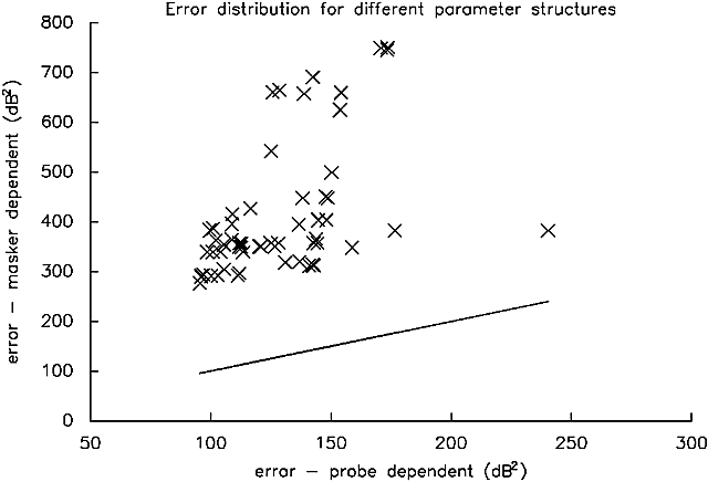
Figure 1. A comparison of the goodness-of-fit of PolyFit models of identical structure, one of which has filter parameters depending upon probe level (abscissa), and one of which has filter parameters depending upon masker level. The goodness-of-fit measure is the sum of the squared residuals; hence, smaller numbers indicate better fits. Only parameter structures resulting in models with a goodness-of-fit less than 1000 dB² are included (a total of 63 comparisons). The solid line indicates equal goodness-of -fit for the two possible dependencies.

Another way to demonstrate this is to compare the fits from the best-fitting probe- and masker-dependent models for various numbers of coefficients. Figure 2 shows, again, the overwhelmingly better fit obtained by making filter parameters depend upon probe rather than masker level.

Although it is quite clear that probe-dependent models are much preferable to masker-dependent models, it is much more difficult to choose a particular probe-dependent model out of the many possible. Clearly, for a fixed number of coefficients to be estimated, one would typically choose the best-fitting model - the difficult issue is the choice of the number of coefficients, and how this trades off against the goodness-of-fit.

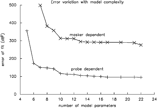
Figure 2. Summary measures of the goodness-of-fit of PolyFit models which fit the data best with a given number of coefficients, for models in which filter parameters depend upon the level of the probe, and of the masker.

To aid us in this task, we have adopted a heuristic approach based on those common in statistical model building (e.g., see Aitkin, Anderson, Francis, & Hinde, 1989). Starting off with a model with more coefficients than we think are necessary, we then determine which can be excised by looking at changes in the goodness-of-fit as they are excised. Unfortunately, for the type of nonlinear model employed here, there is no statistical theory which can assess the statistical significance of any given change in error. Often, however, excising some coefficients hardly changes the error, whereas excising others changes the fit of the model dramatically. In our earlier publication (Rosen & Baker, 1994), we had the good fortune for this to be true consistently. Here, the results are not as clear cut, but as we shall see, models with similar goodness-of-fit lead to filter shapes that are very similar. Therefore, it is not particularly important which model is chosen from the "better-fitting" ones.

First note that a quadratic dependence of all parameters on probe levels leads to little improvement on the fits obtainable from a linear dependence. The quadratic model, with 22 coefficients to estimate (3 for each of the 6 filter parameters and k, plus one for absolute threshold) leads to a fit of 95.6 dB², whereas the linear model, with 15 parameters, leads to a fit of 102.2 dB². Thus a loss of 7 coefficients worsens the goodness-of-fit by only 6.6 dB². Table 2 shows the best-fitting models for a particular number of estimated coefficients. Models are generally described by a letter (p or m indicating probe or masker dependence) followed by a string of 7 digits indicating the number of coefficients used for each of the parameters p_l, p_u, k, w_l, w_u, t_l and t_u, respectively. An 'x' indicates a parameter that is not needed, for example, when only a roex(p) shape is needed on the high-frequency side of the filter. Thus p2212x1x indicates a model in which both lower and upper p depend upon probe level in a linear way, as does w_l, with a simple roex(p) shape on the high-frequency side. All other parameters are invariant across level. A '0', used only for describing filter parameters for the upper half of the filter, indicates that the filter shape has identical values on its high and low frequency sides for that particular parameter. Thus p1012x1x indicates a model with a simple roex(p) shape on its high-frequency side, but symmetric in its passband. Only one filter parameter varies with level (w_l).

Note that it is possible to account reasonably well for the data with as few as 6 coefficients. Of these, two concern absolute threshold and detection efficiency (k), while only 4 describe filter shape (assuming symmetry in the passband - by setting p_u = p_l - did not harm the fit and allowed the loss of one parameter). Only one filter parameter need depend on level (w_l). Also of note is the fact that k can generally be assumed to be invariant across level without affecting the fits obtained. This empirical fact supports a simpler interpretation of our results than would otherwise be the case (see the discussion below).

Table 2. Goodness-of-fit for the best-fitting model containing 5-22 estimated coefficients. All are probe dependent models. The first 7 columns contain the number of polynomial coefficients used for each filter parameter. The last column indicates the difference in the goodness-of-fit measure between the model given by that row, and the model on the row immediately above.

Figure 3 shows the filter shapes, as a function of level, derived from 4 of the models described in Table 2. Although the goodness-of-fit varies by about a factor of two, there is little change evident on the low-frequency sides of the filter. Even the high-frequency sides (which are known to be somewhat difficult to pin down in notched-noise experiments as threshold increases are dominated by the effects of the shallower side of the filters) differ little unless they are not permitted to change with level. So, although there is some uncertainty in choosing a particular model, many of the models which fit the data reasonably well lead to similar conclusions about filter shapes.

We have chosen to focus on p1312x2x, as a further reduction in the number of coefficients leads to a relatively large increase in the sum of the squared residuals, considerably larger than reductions in models with more coefficients. This model appears to be a good compromise among the number of parameters used, the goodness-of-fit, and the 'look' of the resulting filter shapes. Other choices would lead to conclusions little different. The quadratic term for p_u allows the upper slope of the filter to remain relatively constant for low levels, and then to become shallower with increasing level once the probe level reaches about 50 dB SPL. Models in which p_u is constant, or a linear function of level, lead to odd behaviour in the upper tails of the filter; in particular, the tail starts just a few dB down from the peak. Clearly, the roex(p,w,t) was not designed with such a possibility in mind, so it seems far preferable to allow a quadratic dependence in one parameter. In any case, this strategy leads to the best fits for a given number of estimated coefficients.

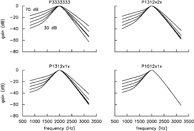
Figure 3. Filter shapes for 4 different probe-dependent models. Each plot shows the filter shapes calculated for probe levels of 30-70 dB SPL in 10 dB steps.

That the models do fit the data quite well can be appreciated from Figure 4, which shows the entire data set, plotted as growth-of-masking functions, along with the predictions from our chosen model. All predictions are within -2.8/+2.0 dB of the obtained data points with a total sum-of-squared residuals being 116.6 dB² over 158 measurements. Contrast this with the predictions from the best masker-dependent model with the same number of estimated coefficients in Figure 5 (m2222x1x). Although in many situations, this would be considered quite a good fit, note the many regions in which the data is consistently predicted poorly. The predictions are only within -5.7/+3.3 dB of the obtained data points with a total sum-of-squared residuals being 313.7 dB², nearly a factor of 3 worse.

There is another way of plotting filter shapes which also points to probe-dependent models being superior. The filter shapes shown above are all normalised to have unity gain at their peak, as a consequence of the assumptions involved in fitting roex filter shapes. Yet we know from direct measurements of basilar membrane vibration that peak gain varies directly with level, being greatest at lowest levels (Ruggero, Rich, & Recio, 1992). Such measurements also show basilar membrane response to be linear for frequencies sufficiently below the best frequency of the place on the membrane being investigated, as shown in Figure 6. Note too the compressive response at the peak of the filter, with a change in gain of about 20 dB for a 40 dB input range.

Working on the hypothesis that our behavioural results reflect basilar membrane filtering in a fairly direct manner, we assume that the auditory filter is linear a little more than one octave below its characteristic frequency, thus tacking together the shapes at this point. The resulting curves are highly reminiscent of filtering functions measured on the basilar membrane, particularly with respect to the way in which filter sharpness and peak filter gain both increase with decreasing level (Figure 7) and for the tendency for the filters to become linear again at frequencies high above CF. The 2:1 compression ratio at the peak is also similar to that evidenced on the basilar membrane. Note too that the filters so calculated change shape right down to absolute threshold. This is to say that the nonlinearity extends to levels as low as it is possible for us to measure. There is some controversy about this, with claims that the basilar membrane is linear even at its peak response for levels below a threshold that can be as high as 30-40 dB SPL. Recent measurements by Nuttall & Dolan (1996) support our view in showing that the response of the basilar membrane does indeed become linear at low enough levels, but only "... for basilar membrane velocities below afferent neural thresholds based on discharge rates" (p 1561).

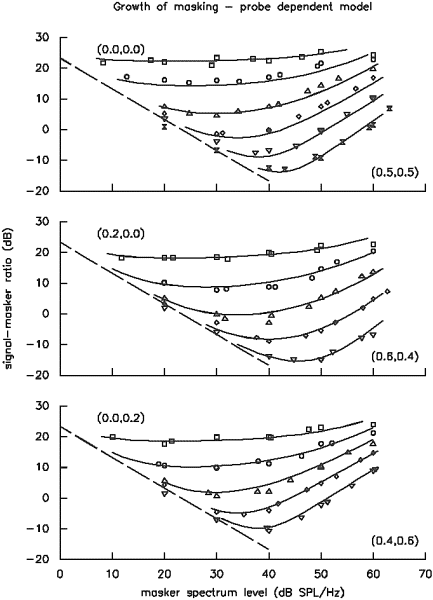
Figure 4. Masked thresholds expressed as signal-to-noise ratios (probe level in dB SPL - masker level in dB SPL/Hz) as a function of masker level. Such curves are typically known as growth-of-masking functions. The results from symmetric notches and the two types of asymmetric notches are shown in separate graphs. Each symbol indicates a particular pair of notches. The lines are predictions from a model which assumes filter parameters to depend upon probe level. The diagonal line at left indicates absolute threshold.

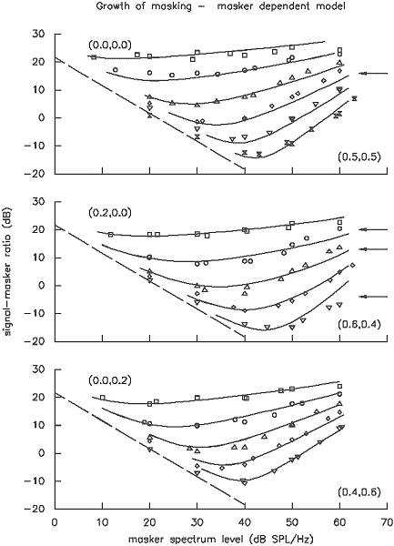
Figure 5. As for Figure 4, but with predictions from a masker-level-dependent model. Arrows indicate regions in which the fit of the model is consistently poor.

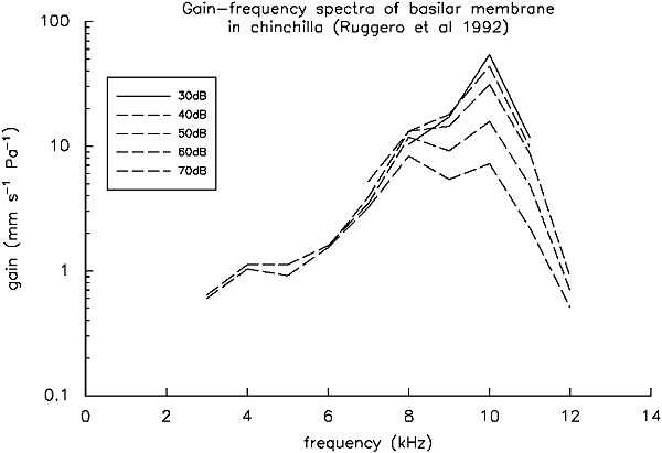
Figure 6. The frequency response of a single place on the basilar membrane as a function of level (redrawn from Ruggero et al., 1992).

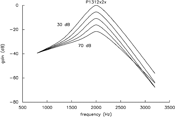
Figure 7. Filter shapes for a p1312x2x probe-dependent model, calculated for probe levels of 30-70 dB SPL in 10 dB steps, and normalised to have equal gain a little more than one octave below their centre frequency.

The same manipulation leads to a much messier picture for the masker-dependent models. Figure 8 shows the filter shapes normalised in both ways. Although the filter does become shallower with level on its low frequency side in the passband, the tail sharpness appears to increase with increasing level. Also, filter sharpness does not turn out to be linked to peak filter gain in the way suggested by basilar membrane experiments.

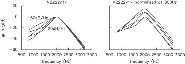
Figure 8. Filter shapes for a m2222x1x masker-dependent model, calculated for masker levels of 20-60 dB SPL in 10 dB steps, normalised both to have equal gain at their tips, and about an octave below their centre frequency.

We have also found that the filter shapes obtained from masker-dependent models change much more with changes in parameter structure, as can be seen in Figure 9. In the m2212222 model, the change in gain is even greater than that in the input level, rather than the 2:1 compression seen on the basilar membrane.

In short, there are strong reasons to prefer models of auditory filtering which make filter parameters depend upon probe level rather than masker level: 1) The probe-dependent models predict the data considerably more accurately, with the sum of the squared residuals 2-3 times larger for masker-dependent models; 2) Probe-dependent models lead to filter shapes much more in keeping with physiological measures. 3) Filter shapes derived from masker-dependent models change greatly with small changes in the parameter structure assumed. Filter shapes derived from probe-dependent models change little even with large changes in the assumed parameter structure.

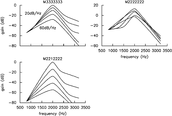
Figure 9. Normalised filter shapes for 3 different masker-dependent models. Each plot shows the filter shapes calculated for masker levels of 20-60 dB SPL in 10 dB steps. Note the strong variation in shapes for different parameter structures.

Normal listeners: Mean of 2. Rosen and Baker (1994) reported similar analyses to those above on a set of mean data from two different listeners. It is interesting to compare the filter shapes from the two sets of mean data from three points of view. First, the listeners in the earlier study had about half of the number of conditions described above (78 averaged from a set of 386 individual thresholds), and it would be interesting to know how much the derived filter shapes depend upon the particular set of conditions used. Second, the earlier study used different apparatus and stimulus generation techniques, and although we do not think this would have made a difference, we would like to be assured. Finally, given the inevitable individual variability, it would be helpful to know how much results are likely to vary across groups of listeners. Figure 10 (corresponding to Figure 7) shows the filter shapes derived from the same probe-dependent model focused on above. It is clear that the two sets of data lead to highly similar imputed filter shapes across level, in spite of all the differences between them.

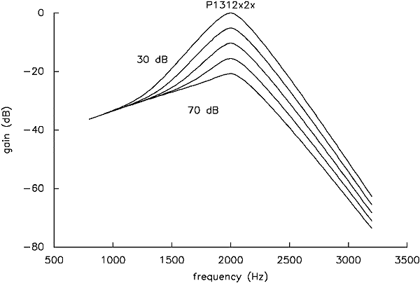
Figure 10. Filter shapes from the data obtained by two normal listeners in Rosen and Baker (1994) - a p1312x2x probe-dependent model, calculated for probe levels of 30-70 dB SPL in 10 dB steps, and normalised to have equal gain at about one octave below their centre frequency. Compare this to Figure 7.

Normal listeners: Individual results. Similar analyses were performed for the individual data sets obtained from each of the listeners. Table 3 shows the goodness-of-fit measures for a selection of models for each individual data set. These measures vary significantly across listeners for at least two reasons. First, listeners participated in varying numbers of conditions, and, all other things being equal, more data points lead to increased overall goodness-of-fit measures. But listeners also differ in their inherent consistency, and we would expect more consistent listeners to have better fits.

Of more interest, in any case, is the pattern of results across conditions within an individual listener. Note first that probe-dependent models always fit the data better than masker-dependent models, typically by a factor of 2-3. In fact, we have never found a case in which a masker-dependent model fits the data better than a probe-dependent model of the same structure (in literally hundreds of comparisons). Secondly, for the probe-dependent model in which all parameters vary linearly with level, there is typically little loss of predictive power in assuming k (signal detector efficiency) to be constant across level. Figure 11 shows the individual normalised filter shapes arising from the p1312x2x model we used above. Again, however, there are a wide variety of parameter structures which lead to similar filter shapes. Clearly, individual listeners differ in their frequency selectivity, but the essential pattern is strikingly uniform.Table 3. Individual measures of goodness-of-fit from a number of PolyFit models. Also shown are results from the Mean-of-3 and Mean-of-2 data sets described above.

Contrast this with the filter shapes that arise from the m2222x1x masker-dependent model discussed above (Figure 12). These are much more variable from listener to listener, both in the degree of compression (or even expansion) across level, and even in which level leads to the highest gain.

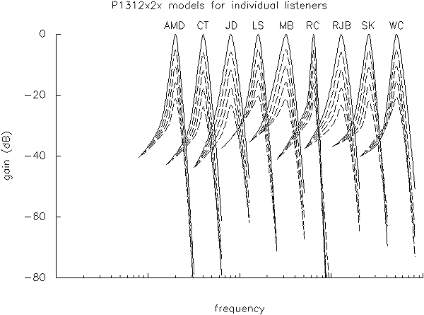
Figure 11. Filter shapes for 9 normal-hearing listeners using a p1312x2x probe-dependent model, calculated for probe levels of 30-70 dB SPL in 10 dB steps, and normalised to have equal gain at just less than one octave below their centre frequency. The curves have been shifted in logarithmic frequency axis for clarity.

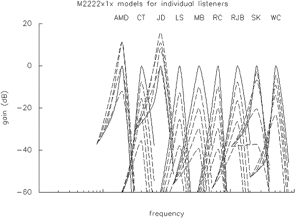
Figure 12. Filter shapes for 9 normal-hearing listeners using an m2222x1x masker-dependent model, calculated for masker levels of 20-60 dB SPL in 10 dB steps, and normalised to have equal gain at just less than one octave below their centre frequency (cf. figure 11)

Hearing-impaired listeners. Growth of masking functions obtained from listener ET are shown in Figure 13. Note how the functions are essentially parallel, indicating that filter shapes do not change with level. Auditory filtering in ET thus appears to be linear, quite unlike that found in any normal listener. The upward slope of the functions indicates that k (the measure of signal-detection efficiency) is increasing with level. Although such a trend clearly does not occur in the mean data from normal listeners analysed above, some normal listeners do show evidence of k increasing with level. Although this is an issue that needs further exploration, suffice it to say for now that ET is the only listener in whom variations in k can substantially account for changes in masking across level. Therefore, using the heuristic techniques described above for selecting an appropriate model results in a simple roex(p) shape with k a linear function of probe level (p112).

CH, the other listener with a minor hearing impairment, shows a pattern intermediate to that exhibited by ET and the normal listeners. Although his growth of masking functions are considerably more parallel then normal listeners, they do show some convergence as level increases (Figure 14). His data is poorly fit by a model which assumes filtering not to change with level (that is, linearity), even if k is allowed to vary with level. A good fit can, however, be obtained with a simple model which is symmetric in the passband, and has only w_l changing with level - p1012x1x. Note too from Table 3 that the advantage of the probe-dependent models is somewhat reduced with the reduced filter nonlinearity exhibited by CH, just as would be expected. Interestingly, even the model for ET with only a k dependence on level performs better on the basis of probe level as opposed to masker level (103.0 vs. 140.2 dB²). This must have implications for the nature of the signal-detection process.

Plots of normalised filter shapes from these two listeners, compared to the mean of 3 analysed above, confirm the main findings just pointed out: ET shows a complete lack of nonlinearity, while CH shows a degree of nonlinearity intermediate between ET and the normal listeners (Figure 15). Another feature becomes evident in this comparison. Both ET and CH show a degree of frequency selectivity comparable to normal listeners at high levels. The degradation of frequency selectivity only becomes apparent at lower levels, because their filters sharpen little or not at all with decreasing input level.

This result is consistent with the notion that the changes in threshold and selectivity (including the reduced variation in filter shape with level) can be attributed purely to damage to outer hair cells, which are believed to be the source of basilar membrane nonlinearity (see Patuzzi & Robertson, 1988 for a review). In this view, inner hair cells operate primarily as sensory transducers, but have no direct effect on basilar membrane vibration. Outer hair cells modulate basilar membrane vibration (by a mechanism that is still the subject of much controversy), making it nonlinear. As level increases, however, and vibration becomes greater, the outer hair cells exert less and less effect, resulting in a linear vibratory response at sufficiently high levels. By the same token, if the outer hair cells are absent, the membrane vibrates linearly at all levels. Outer hair cells that are damaged only partially lead to an intermediate degree of nonlinearity. There is strong supporting evidence for this idea in a series of experiments by Ruggero and his colleagues showing basilar membrane vibration patterns to become linear at high levels, with ototoxic poisoning, and with the death of the animal (Ruggero & Rich, 1991; Ruggero et al., 1992; Ruggero, Rich, & Recio, 1993), coupled with the fact that the outer hair cells appear to be much more physiologically vulnerable than the inner hair cells. In short, it appears that the primary cause of the hearing impairment exhibited by our two listeners arises solely or primarily from outer cell damage.

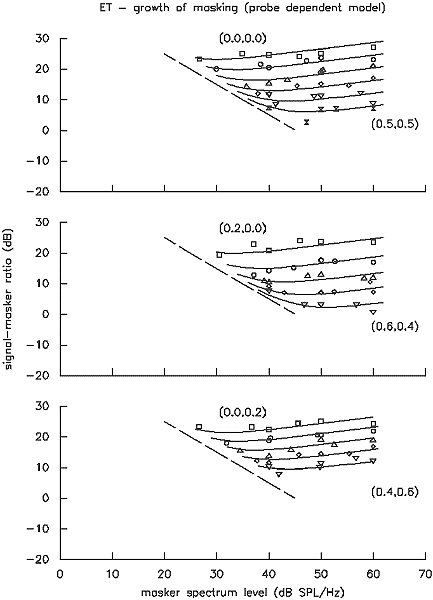
Figure 13. Growth-of-masking functions (analogous to those shown in Figure 4) for listener ET, along with the predictions of a p112 model.

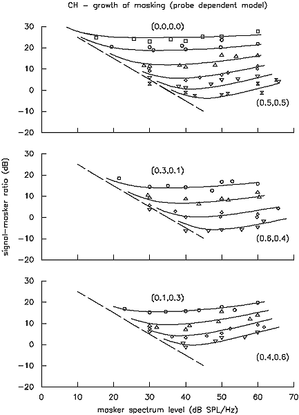
Figure 14. Growth-of-masking functions for listener CH, along with the predictions of a p1012x1x model.

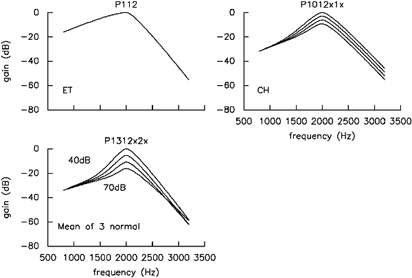
Figure 15. Normalised filter shapes from hearing-impaired listeners ET and CH with appropriate comparison shapes (probe levels from 40 to 70 dB SPL in 10 dB steps).

4. Summary and final remarks
We have shown that it is possible to accurately account for the pattern of results across level in a notched-noise masking experiment with filter shape models that explicitly depend upon probe level. Such models have relatively few parameters, yet lead to results that are highly reminiscent of vibration patterns observed directly on the basilar membrane. Therefore, notched-noise measurements which are made only at one level should be performed with a fixed probe level. Fixing the masker level leads to an imputed filter shape that is some kind of average of a number of shapes, caused by the change in probe level as notches are varied. In general, such filter shapes will be too narrow, simply because the filter is becoming sharper as the probe level decreases with increasing notch width.

There is still much to be done regarding the computational implementation of nonlinear filters that have these properties, in order to produce a general-purpose nonlinear auditory filter bank. In terms of the distinction between "input" vs. "output" control of filter shape (Lutfi & Patterson, 1984; Verschuure, 1981), our results clearly support the notion that the filter shape is controlled by its output level. This arises from the finding that k appears to be constant across level, so that fixing the probe level also fixes the output level of the filter. On the other hand, it may well be that filter structures that are neither directly input- nor output-controlled lead to results consistent with our findings (e.g., the MBPNL model of Goldstein, 1988). Explicit models of auditory filtering will also be necessary for detailed comparisons of basilar membrane data with psychophysical results, preferably obtained in the same species.

We have also successfully applied our technique to two hearing-impaired listeners, leading to results that unambiguously indicate damage to the outer hair cells. Pure outer hair cell damage would be expected to manifest itself in four linked ways relevant to the discussion here: 1) a loss of absolute sensitivity; 2) smaller or no changes in filter shape across level; 3) degraded selectivity at low levels; and 4) normal selectivity at sufficiently high levels. All 4 of these features are clearly displayed in the results above. Further work in this area will focus on a variety of manifestations of auditory nonlinearity (including otoacoustic emissions), with the goal of determining to what extent an even wider variety of phenomena can be accounted for by a single mechanism.

5. Acknowledgements
This work was supported by the Wellcome Trust and the MRC. Thanks to Sarah Kramer and Rosie Casson who collected some of the data reported here, and also to Alberto Recio who provided the data for figure 6.

6. References
Aitkin, M., Anderson, D., Francis, B., & Hinde, J. (1989). Statistical modelling in GLIM. Oxford: Clarendon Press.

Goldstein, J. L. (1988) Updating cochlear driven models of auditory perception: A new model for nonlinear auditory frequency analyzing filters. In B. A. G. Elsendoorn & H. Bouma (Eds.), Working Models of Human Perception (pp. 19-57). London: Academic Press.

Lutfi, R. A., & Patterson, R. (1984) On the growth of masking asymmetry with stimulus intensity. Journal of the Acoustical Society of America, 76, 739-745.

Moore, B. C. J., & Glasberg, B. R. (1987) Formulae describing frequency selectivity as a function of frequency and level, and their use in calculating excitation patterns. Hearing Research, 28, 209-225.

Nuttall, A. L., & Dolan, D. F. (1996) Steady-state sinusoidal velocity responses of the basilar membrane in guinea pig. Journal of the Acoustical Society of America, 99, 1556-1565.

Patterson, R. D., & Moore, B. C. J. (1986) Auditory filters and excitation patterns as representations of frequency resolution. In B. C. J. Moore (Ed.), Frequency Selectivity in Hearing. London: Academic Press.

Patterson, R. D., Nimmo-Smith, I., Weber, D. L., & Milroy, R. (1982) The deterioration of hearing with age: Frequency selectivity, the critical ratio, the audiogram, and speech threshold. Journal of the Acoustical Society of America, 72, 1788-1803.

Patuzzi, R., & Robertson, D. (1988) Tuning in the mammalian cochlea. Physiological Review, 68, 1005-1082.

Rosen, S. (1989) Deriving auditory filter characteristics from notched-noise masking data: Modified derivations. Speech, Hearing and Language: Work in Progress, 3, 189-204.

Rosen, S., & Baker, R. J. (1994) Characterising auditory filter nonlinearity. Hearing Research, 73, 231-243.

Rosen, S., & Fourcin, A. J. (1986) Frequency selectivity and the perception of speech. In B. C. J. Moore (Ed.), Frequency Selectivity in Hearing (pp. 373-487). London: Academic Press.

Ruggero, M. A., & Rich, N. C. (1991) Furosemide alters organ of Corti mechanics: Evidence for feedback of outer hair cells upon the basilar membrane. The Journal of Neuroscience, 11(4), 1057-1067.

Ruggero, M. A., Rich, N. C., & Recio, A. (1992) Basilar membrane responses to clicks. In Y. Cazals, L. Demany, & K. Horner (Eds.), Auditory Physiology and Perception (pp. 85-91). Oxford, U.K.: Pergamon Press.

Ruggero, M. A., Rich, N. C., & Recio, A. (1993) Alteration of basilar membrane responses to sound by acoustic overstimulation. In H. Duifhuis, J. W. Horst, P. van Dijk, & S. M. van Netten (Eds.), Biophysics of Hair Cell Sensory Systems (pp. 258-265). Singapore: World Scientific.

Verschuure, J. (1981) Pulsation patterns and nonlinearity of auditory tuning II. Analysis of psychophysical results. Acustica, 49, 296-306.

West, P. D. B., & Evans, E. F. (1990) Early detection of hearing damage in young listeners resulting from exposure to amplified music. British Journal of Audiology, 24, 89-103.

Zwicker, E., Terhardt, E., & Paulus, E. (1979) Automatic speech recognition using psychoacoustic models. Journal of the Acoustical Society of America, 65, 487-498.

© 1996 Stuart Rosen, Richard J. Baker and Angela Darling.

Back to Publications

Back to Phonetics and Linguistics Home Page