

1. Introduction
Hidden Markov models (HMMs) have proved to be a very successful
approach to automatic speech recognition. In addition to providing
a tractable mathematical framework with straightforward algorithms
for training and recognition, HMMs have a general structure which
is broadly appropriate for speech (Holmes and Huckvale, 1994).
In particular, the time-varying nature of spoken utterances is
accommodated through an underlying Markov process, while statistical
processes associated with the model states encompass short-term
spectral variability. The approach does however make assumptions
which are clearly inappropriate from a speech-modelling viewpoint.
The independence assumption states that the probability
of a given acoustic vector corresponding to a given state depends
only on the vector and the state, and is otherwise independent
of the sequence of acoustic vectors preceding and following the
current vector and state. It is also assumed that a speech pattern
is produced by a piece-wise stationary process with instantaneous
transitions between stationary states. The model thus takes no
account of the fact that a speech signal is produced by a continuously
moving physical system (the vocal tract).
The inappropriate assumptions of HMMs can be considerably reduced by using a segment-based approach (see Ostendorf, Digalakis and Kimball, 1996, for a review). A segment-based model represents sequences of several consecutive acoustic feature vectors and can therefore explicitly characterise the relationship between these vectors. One such approach is being developed at the Speech Research Unit, DRA Malvern. The HMM formalism is being extended to develop a dynamic segmental HMM (Russell, 1993; Holmes and Russell, 1995b), which overcomes the limitations while retaining the advantages of the general HMM approach. The goal is to provide an accurate model for variability between sub-phonemic speech segments, together with an appropriate description of how feature vectors change over time during any one segment. In addition to the general aim of improving recognition performance, this approach can provide insights into the nature of speech variability and its relationship with acoustic modelling for speech recognition.
The experiments described in the current paper have involved analyses of natural speech data in order to investigate how well the data fits the modelling assumptions of the segmental HMM, independently of any one particular set of trained segmental models. Studies have been carried out of both the pattern of feature vectors over the duration of a segment and the variability across different segments. Section 2 provides some background by briefly introducing segmental HMMs and explaining the underlying model of speech variability. Section 3 then describes the general experimental framework for analysing speech data according to the segmental model, and the experiments themselves are discussed in the following sections.
2. Segmental HMMs
An important concept in segmental HMMs is the idea that the relationship
between successive acoustic feature vectors representing sub-phonemic
speech segments can be approximated by some form of trajectory
through the feature space. A segmental HMM for a speech sound
provides a representation of the range of possible underlying
trajectories for that sound, where the trajectories are of variable
duration. Any one trajectory is considered to be "noisy",
in that an observed sequence of feature vectors will in general
not follow the underlying trajectory exactly. For reasons of
mathematical tractability and of trainability, the trajectory
model is parametric and all variability is modelled with Gaussian
distributions assuming diagonal covariance matrices. There are
two types of variability in the model: the first defines the extra-segmental
variations in the underlying trajectory, and the second represents
the intra-segmental variation of the observations around
any one trajectory. Intuitively, extra-segmental variations represent
general factors, such as differences between speakers or chosen
pronunciation for a speech sound, which would lead to different
trajectories for the same sub-phonemic unit. Intra-segmental
variations can be regarded as representing the much smaller variation
that exists in the realisation of a particular pronunciation in
a given context by any one speaker.
The probability calculations with segmental models apply to sequences of observations and therefore involve considering a range of possible segment durations. It is thus possible to incorporate explicit duration modelling, by assigning probabilities to each segment duration (with the durations specified as the number of 'frames' of feature vectors). However, this paper concentrates on the acoustic modelling and any duration probability component is therefore ignored in the discussions of probability calculations.
Considering a segment of observations  and a given state of a Gaussian segmental HMM (GSHMM), the joint
probability of y and a trajectory fa
is specified by the equation

where P( fa ) represents the extra-segmental
probability of the trajectory given the model state, and  represents
the intra-segmental probability of the observations given the
trajectory. Although the individual observations in y are
treated independently, the dependence on the trajectory fa
provides a strong constraint due to its relatively small variance.
This is a major advantage over conventional HMMs, which treat
all observations for all examples represented by any one state
in the same way.
The probability of the segment y given the segmental HMM
state can be obtained by integrating (or summing) the trajectory
probabilities over the set of all trajectory parameters. An alternative
is to consider only the optimal trajectory, whose parameters
are those which maximise the joint probability .
It is straightforward to derive the optimal trajectory, given
a segment of data and a state of a GSHMM. Considering only the
optimal trajectory has the advantage that the mathematics associated
with segmental models is simplified, and also that it is easy
to study the model representation of particular speech segments.
The analyses described in this paper, and the experiments which
have so far been conducted at the Speech Research Unit, are all
based on the optimal trajectory approach. The exact form of the
optimal trajectory model depends on the trajectory parameterisation
which is adopted. The simplest case is a static segmental HMM
(Russell, 1993), where the underlying trajectory is assumed to
be constant over time and is thus represented by a single "target"
vector. By assuming that the underlying trajectory changes linearly,
a linear dynamic segmental HMM can be formulated (Holmes and
Russell, 1995b). These two types of segmental HMM have formed
the basis for our experiments, and are described in more detail
below.
2.1 The static model
The static segmental HMM does not attempt to model dynamics, but
does model variability due to long-term factors separately from
variability that occurs within a segment. The impact of the independence
assumption is thus reduced by fixing the long-term factors for
the duration of any one segment. This model represents the simplest
form of segmental HMM and has for this reason been valuable for
understanding the general properties of this segmental approach.
The static model is useful for studying the effect of distinguishing
intra- and extra-segmental variability separately from the effect
of modelling dynamics, and forms a baseline for comparisons with
dynamic models.
Considering a particular state of a static GSHMM, extra-segment
variation is characterised by a Gaussian pdf  ,
which represents the distribution of possible targets for the
segment. Any one target is described by a Gaussian pdf with fixed
intra-segment variance
  . It is thus assumed
that the variability around the target is the same for all targets
and for all observations in all segments corresponding to this
state. The probability of a particular sequence of observation
vectors
  , is defined as

where  denotes the optimal target, which
is the value of the target c that maximises the probability
of y. It can be shown that the value of
  is given by
 .
.
The optimal target  is thus a weighted
sum of the average of the observed feature vectors and the expected
value of the target as defined by the model. The weightings of
these two components are determined by the relative magnitudes
of the extra-segmental and intra-segmental variances. In practice,
 will be strongly biased towards the observations
because the intra-segmental variance will generally be much smaller
than the extra-segmental variance.
2.2 The linear model
A simple dynamic model is one in which it is assumed that the
underlying trajectory vector changes linearly over time. A trajectory
 is defined by its slope m
and the segment mid-point value c, such that
  .
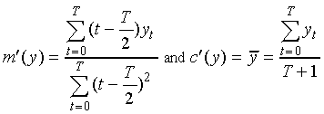
It is well known that the slope m´(y) and mid-point
value c´(y) of the linear trajectory which provides
the best fit to the data y (in a least-squared error sense)
are given by:
 .
.
Now suppose that the distribution of the two trajectory parameters
for a given state is defined by Gaussian distributions  and
and
 (with diagonal covariance matrices) for
the slope and mid-point respectively. The intra-segmental distributions
are assumed to be Gaussian with diagonal covariance matrix .
Ignoring any duration-probability component, the probability of
the sequence y given a particular Gaussian segmental HMM
(GSHMM) can be defined as

where  and
and  are
the values of the slope and mid-point which together maximise
the joint probability of the observations and the trajectory.
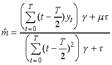
The equation for the optimal mid-point
  has the same form as that for the optimal target in the constant-trajectory
model, and the optimal slope
  is also
a weighted sum of the parameters which are optimal with respect
to the data and their expected values as defined by the model,
thus:
 .
.
As with the constant-trajectory model, the intra-segmental variance will generally be much smaller than the extra-segmental variances, so the optimal trajectory will be biased towards the best fit to the data.
2.3 Studying variability in and around trajectories
The GSHMMs described above make four important assumptions about
the characteristics of acoustic feature vectors representing speech
data, thus:
The corresponding assumption in a conventional HMM (using single Gaussian distributions) is that the variability of all observations in all examples of a segment is Gaussian.
The current studies used natural speech data to investigate the validity of the GSHMM assumptions, and compare them with those of conventional HMMs. The aim was to investigate the characteristics of the data independently from the parameters of particular sets of models. In order to study a GSHMM-type representation of the data, it is necessary to make an estimate of the optimal trajectory. A reasonable approximation to the optimal trajectory was obtained by computing the best fit to the data which, as explained above, should be quite close to the "optimal" value as defined by a model for the segment. For data which is accurately represented by a particular model, the expected value as predicted by the model will be very close to the best fit to the data (and hence also to the optimal value).
3. Experimental framework
The aim of these investigations was to analyse acoustic features
as they would be characterised by a set of simple segmental HMMs.
The "segments" therefore corresponded to the sub-phonetic
units which are represented by HMM states in a typical HMM recogniser.
A simple modelling task was chosen, with mel cepstrum features
representing connected digit data modelled by context-independent
"monophone" models with three states per phone. A set
of conventional HMMs was trained for this task, to provide a basis
for studying the acoustic characteristics of the speech segments
corresponding to each of the HMM states. The details of the task,
the model set and the experimental method are described below.
3.1 Speech data
The analysis of data characteristics was performed on the training
data for the connected-digit task. These data were from 225 male
speakers, each reading 19 four-digit strings taken from a vocabulary
of 10 strings. The test data used in recognition experiments
was taken from 10 different speakers, each reading four lists
of 50 digit triples. The speech was analysed using a critical-band
filterbank at 100 frames/s, with output channel amplitudes in
units of 0.5 dB, converted to an eight-parameter mel cepstrum
and an average amplitude parameter.
3.2 Conventional HMM set
The conventional HMMs used three-state context-independent monophone
models and four single-state non-speech models (for silence and
other non-speech noises such as breath noise), all with single-Gaussian
pdfs and diagonal covariance matrices. The model means were initialised
from a very small quantity of hand-labelled data (three of the
four-digit strings for each of two speakers), and the variances
were all set to the same arbitrary value. For the very limited
context coverage provided by the digit data, initialising the
model means in this way was found to be important to help ensure
that the training alignment of the states to the data was phonetically
appropriate. The models were then trained automatically with
five iterations of Baum-Welch re-estimation. These models gave
a word error rate of 8.2% on the connected-digit test set.
3.3 Method
In order to estimate feature-vector trajectories, it was necessary
to define segment boundaries by labelling the data at the segment
level. An appropriate labelling was obtained by using the above
set of trained three-state-per-phone standard HMMs to perform
a Viterbi alignment to associate each speech frame (represented
by an acoustic feature vector) with a single model state. This
process effectively extracts segments from the data, and distributions
of the durations of the segments were plotted (see Section 4).
For all segments identified in the alignment, a model representation
of the acoustic features was derived for the modelling assumptions
of both the static and linear segmental HMM and, for comparison,
the conventional HMM. For the conventional HMM, all frames corresponding
to a particular state are treated identically, so the model representation
is simply the average of all these frames and is therefore the
same for all segments corresponding to any one state. In the
case of the segmental models, an optimal trajectory vector was
estimated for each individual example as the average of the observed
feature vectors for the static model and as the best-fitting straight
line parameters for the linear model. It was then possible both
to study the trajectory approximations (Section 5) and to analyse
the variability associated with the trajectory model (Section
6).
4. Duration distributions
4.1 Method
For each sub-phonemic speech segment, a count was made of the
number of examples with each possible duration from one frame
up to the maximum which was observed. The resulting histograms
showing number of occurrences against duration were then plotted.
These histograms were useful to assist in interpreting the acoustic
analyses described in the following sections.
4.2 Results and discussion
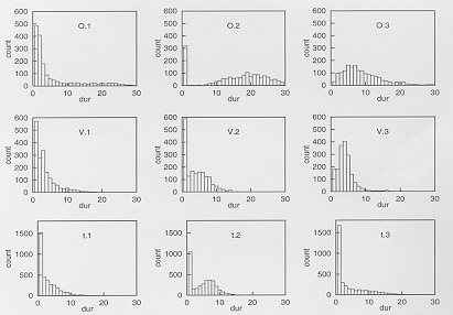
Figure 1 shows representative plots of duration distributions
for the three states of each of three phones. The most striking
characteristic of these distributions is the high proportion of
single-frame segments. From the individual file alignments (see
Figure 2 for an example), it was evident that this characteristic
reflects a tendency for the most likely HMM state alignment path
to use just one of the three available states to represent most
frames within a phone, with the other states being occupied for
the minimum duration of one frame. The implication is that in
some cases the different HMM states in the sequence representing
a phone are in fact being used to model the different acoustic
properties of different examples of that phone, rather than the
pattern of change over any one example. This is not surprising
as the extent of change over the duration of any one example of
a segment may often be less than the difference between different
examples.
Another interesting observation from the duration distributions
is that some of the segment durations are unrealistically long,
even allowing for the fact that some are representing almost a
complete phone in a single 'segment'. These unrealistic distributions
only arise for phones occurring at the ends of words (for example,
 and
and  ,
and not for those (such as
  )
which only occur in the middle of a word. This property reflects
the ability of HMMs to show repeated self-loop transitions in
a state if the end of a word model provides a closer match to
the data than a silence or noise model, even after the utterance
articulation has actually finished.
The above characteristics of the HMM duration distributions are relevant when considering an appropriate range for allowed segment durations in a corresponding set of segmental HMMs. For practical reasons, it is necessary to impose some plausible upper limit on segment duration, which will effectively disallow some of the extremely long durations seen with the conventional HMMs. The range of segment durations should therefore be more plausible, but there may also be problems for instances where the characteristics of observed speech frames are not compatible with a "sensible" segmentation.
 (O.1, O.2, O.3),
  (V.1, V.2, V.3) and
  (t.1, t.2, t.3)
5. Trajectory fits to speech data
5.1 Method
The aim of the experiments described in this section was to obtain
an indication of the ability of static and linear trajectory models
to describe typical observed feature vector sequences within segments.
The studies were therefore based on a small subset of the data,
using a few examples of each digit. For each of the eight cepstrum
features and for the average amplitude feature, the frame-by-frame
observed values were plotted superimposed on the calculated model
values and time-aligned with the segment labels and filterbank
output. The approximations were compared for the three types
of model.
5.2 Results and discussion
Some example plots for the three model types are shown in Figure
2. It can be seen that the conventional HMM approach (Figure
2a) follows the general characteristics of each speech sound,
but that an average over all frames of all examples is often quite
a poor match for any one particular frame. By incorporating the
static segmental modelling assumptions (Figure 2b), individual
examples are matched more closely. When the linear model is applied
(Figure 2c), the model generally follows the pattern of change
of the observed feature vectors very well. For the overall energy
feature and for the lower-order cepstral features, the match to
the frame-by-frame observed values is remarkably close. The higher-order
cepstral features (from around the sixth upwards) tend to change
less smoothly and there is therefore some loss of detail in the
linear approximation.
Overall, it can be concluded from the trajectory plots that, not surprisingly, a dynamic model is necessary to follow the time-evolving nature of acoustic features. It appears that, for models with three segments per phone using mel cepstrum features, a linear model should be adequate to capture the characteristics of these changes, especially as any additional variation around the linear trajectory will be modelled by the intra-segmental variance. The adequacy of a linear model for this modelling task is supported by Digalakis (1992), who demonstrated that a linear assumption is sufficient to explain a high percentage of the dependency between successive observations within a segment. On the other hand, Deng, Asmanovic, Sun and Wu (1994) have argued for the use of higher-order polynomials, although their linear models used no more than two states per phone. A higher-order polynomial should allow less states to be used to represent each phone and hence make greater use of the segmental-model constraints, but the current studies suggest that a linear model makes a good starting point.
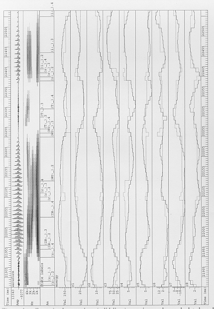
Figure 2a - Frame-by-frame values (solid lines) superimposed on calculated model values as represented by standard HMM modelling assumptions (dotted lines). The tracks are mel cepstrum features for the digit sequence "zero three", time aligned with the speech waveform, filterbank analysis and phone-state labels.

Figure 2b - Frame-by-frame values (solid lines) superimposed on calculated model values as represented by static segmental HMM modelling assumptions (dotted lines). The tracks are mel cepstrum features for the digit sequence "zero three", time aligned with the speech waveform, filterbank analysis and phone-state labels.

Figure 2c - Frame-by-frame values (solid lines) superimposed on calculated model values as represented by linear segmental HMM modelling assumptions (dotted lines). The tracks are mel cepstrum features for the digit sequence "zero three", time aligned with the speech waveform, filterbank analysis and phone-state labels.
6. Distributions describing segmental variability
6.1 Method for computing distributions
Based on the segmentation of the entire training corpus, distributions
of the speech feature vectors were estimated for each model state.
Standard-HMM distributions were calculated, as well as extra-segmental
and intra-segmental distributions for both types of segmental
model. To derive a distribution for any one feature, the range
of possible values for that feature was divided into a fixed number
of sub-ranges or "bins", and the number of occurrences
falling within each bin was counted. In order to make direct comparisons
of variability, the standard-HMM distributions, the extra-segmental
distributions for targets/mid-points and the intra-segmental distributions
were all plotted using the same bin sizes. The bin size for a
given feature was chosen to be appropriate to cover the full range
of values for the feature, using 50 bins. The trajectory slopes
show a very different range of possible values and so the grouping
was different for these distributions. For all distributions,
the Gaussian assumption was evaluated by comparing the observed
distribution with the corresponding best Gaussian fit.
For the standard HMM, distributions were simply accumulated over all frames in all examples of a segment. For the GSHMMs, both extra- and intra-segmental distributions were computed with reference to the trajectory fits for the observed segments. For each state it was then possible to calculate distributions of trajectory parameters: segment averages ("targets") for the static model, and mid-points and slopes for the linear model. The distributions of the mid-points are obviously the same as those of the static model targets. Single-frame segments did not contribute to the slope distributions, which is in accordance with the linear GSHMM probability calculations. For both static and linear models, the distributions of differences between individual trajectories and the observed feature values for each example of each segment were also calculated, to show intra-segmental variability. In order to investigate the effect of segment duration on the observed distributions for the segmental models, distributions were studied for specific segment durations as well as for all examples of a segment combined irrespective of duration.
6.2 Results and discussion
6.2.1 General observations of phone-dependent characteristics
The means of the distributions of the observed features were generally
quite distinct for the different phones, although the extent of
the variability is such that there is inevitably considerable
overlap between the different distributions. Figure 3 shows a
few examples for the first two cepstral coefficients. For the
monophthong  ,
there are only quite small differences between distributions for
the three states. The situation is similar for the fricative
 , although the distributions for the last state show considerably
greater variability than for the other two states, presumably
because the representation includes quite different contexts ("four"
and "five"). The stop consonant
  shows somewhat
greater variability, both in each individual distribution and
across the three states.
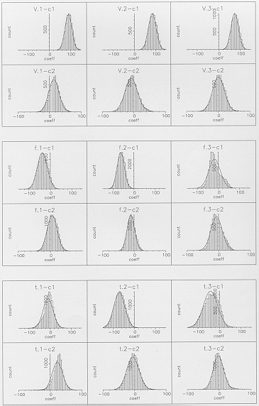
Figure 3 - Distributions illustrating total variability
(as represented by a conventional HMM) of the first two cepstral
coefficients for the three states of  (V.1, V.2, V.3),
  (f.1, f.2, f.3) and
  (t.1, t.2, t.3).
6.2.2 Effect of separating two types of variability
Figure 4 shows typical distributions for the two types of segmental
model, representing variability of the first two cepstral coefficients
for the middle state of  and for the final state of
  . By comparing the segmental models
with the conventional HMM (Figure 3), it can be seen that the
extra-segmental variability of the targets or mid-points across
different segments is of a similar magnitude to the total variance
as represented by the HMM. The intra-segmental variance is however
considerably less than the total variance, and so a GSHMM will
provide a greater constraint on the extent of within-segment frame-to-frame
variability than is possible with a conventional HMM representing
all variability within a single distribution. Comparing the linear
model with the static form demonstrates the benefits of incorporating
dynamics, as the intra-segmental variability is considerably smaller
and hence the effect of the independence assumption will be further
reduced.
6.2.3 Extra-segmental variability
In most cases, the extra-segmental distributions of the targets/mid-points
were strikingly well-modelled by single Gaussians (see Figure
4a for a typical example). There were a few for which the single
Gaussian was not very accurate, such as the third segment of  (Figure 4b), but overall it appears that the assumptions of the
extra-segmental model for the targets/mid-points are quite good
for these data. The sounds for which the single Gaussian appeared
less appropriate are those such as
  which occurs in two quite
different contexts in the digit data. There will also be considerable
variation between different examples for the
  in "eight",
depending on the following sound.
Example target/mid-point distributions of the first and second cepstral coefficients are shown in Figure 5 for individual segment durations ranging from one to five frames. All these distributions show similar variance with the shapes of the distributions appearing generally appropriate for Gaussians, given the numbers of samples in the individual distributions. It therefore seems, at least for the digit data examined in these experiments, that it is a reasonable assumption that the extra-segmental variability of the optimal targets or mid-points of any one feature can be described by a single Gaussian, irrespective of segment duration.
Example extra-segmental distributions for the linear model slopes
(computed over all segment durations) are included in Figure 4.
The single-Gaussian approximation for the slope distributions
was generally not so good as for the mid-point distributions,
although it was much worse for some segments (such as the last
segment of  shown in Figure 4b) than for others (such as the
middle segment of
  shown in Figure 4a). For segments such as the
  , problems appear
to be caused by a small proportion of segments having a feature
slope which is very far from the mean value. From Figure 6b,
showing slope distributions for
  with each segment duration
treated individually, it is evident that this problem is largely
due to difficulties in reliably computing a representative slope
for short segment durations. This difficulty did not occur for
all segments (see for example the plots for the middle segment
of
  , shown
in Figure 6a), and it seems that there are only serious problems
for very short segments of three frames or less. This effect
should be less when using the optimal trajectory rather than the
best data fit, but is still likely to be a problem due to the
bias of the optimal trajectory towards the data. It does therefore
appear that special treatment may be required for very short segments,
in order to obtain robust and general slope distributions as a
basis for the model representations. As the cepstral parameters
mostly change quite smoothly, one possibility is to compute the
trajectories over a wider window which should give a more reliable
estimate of underlying trends.
6.2.4 Intra-segmental variability
The intra-segmental distributions also show some interesting patterns.
There were some differences between different speech sounds,
but typical examples for two model states are included in Figure
4 for both the static and linear models. It is evident that the
observed feature values for a high proportion of the frames are
very close to their mean, with higher and lower values being much
less probable. This effect is the greatest for the linear model,
where the trajectories will generally fit the observations more
closely. The best single-Gaussian fits to the intra-segmental
distributions are obviously not very good, as they will not give
a high enough probability to close matches to the mean while also
tending not to give sufficient penalty to deviations away from
the mean. The shapes of the intra-segmental distributions suggest
that there will be a problem with representing this variability
with a single-Gaussian model. The problem is evidently worse
for some sounds than others: in the examples shown in Figure 4,
the final segment of  is much worse than the middle segment
of
  .
.
Segment duration will obviously affect the calculated intra-segmental
distributions. With the distributions as calculated here, the
static model fits single-frame segments exactly, and the linear
model also provides a precise match for two-frame segments. The
effect of segment duration on the observed intra-segmental variability
can be seen by studying the distributions for each segment duration
individually. An example is shown in Figure 7, for the static
segmental representation of the final segment of  , for which
there are plenty of examples at each of the durations between
two and eight frames. A distribution is not plotted for a duration
of one frame as this is obviously just a spike at zero. Not
surprisingly, the extent of the variability increases with segment
duration, although for durations of three frames and longer the
duration-dependent distributions are actually quite similar to
each other. The single-Gaussian approximations to these individual
distributions are much closer than for the combined distribution,
but still show a tendency to underestimate the probability of
very close fits to the trajectory. The really poor fit of the
single Gaussian when taken over all durations for segments such
as the
  example is largely explained by the single-frame segments,
which form a high proportion of the total number of segments (refer
to Figure 1). In fact, by plotting distributions for all segments
except those of only one frame, the shapes are considerably nearer
to Gaussian.
The shapes of the intra-segmental distributions are a consequence of the well-known problem of estimating a population mean and variance from a small sample of data. As the majority of the segments are quite short (considerably less than 10 frames long, with many being only one frame long), estimates of the mean which are taken from the data will be biased towards those data. When this mean is then used as the basis for estimating the variance of the observations, there will be a tendency to underestimate the variance. The extent of this problem depends on the segment duration. The issue is particularly problematic when the distributions are calculated from the data only, but also applies to the optimal trajectory segmental model as the trajectory still depends on the data. Ideally, the segmental HMM probability calculations should overcome or somehow take into account this duration-dependent bias in the measured variance. From a practical viewpoint however, some method of dealing with very close matches to the mean may be sufficient, as the Gaussian model does not seem unreasonable for the remainder of the distribution. Using the simple Gaussian segmental model as a starting point, distributions have been observed for trained sets of models and the relation with recognition performance has been studied (Holmes and Russell, 1996).
7. Note on recognition performance
This paper is not primarily about recognition experiments, but
some of the major findings so far are briefly summarised here,
as they can be related to the studies of the data which have been
described in the preceding sections. The early recognition experiments
concentrated on establishing the approach with a basic system
which used the same underlying model structure as is typically
used with conventional HMMs: three-state models including self-loop
transitions. The models were therefore given flexibility in represent
each example of a phone by any number of "segments",
and the modelling was restricted to short segments. Within this
framework, the ability of the trajectory-based segmental approach
to improve recognition performance was established for static
models (Holmes and Russell, 1995a) and then to a greater extent
for linear models (Holmes and Russell, 1995b).
The next stage was to progress to models without self-loops and hence a smaller number of segments per phone so that it was necessary to represent extra- and intra-segmental variability in segments with a wider range of durations. Such models correspond most closely with the data analyses which have been described in this paper. The recognition experiments have so far concentrated on the static model (Holmes and Russell, 1996). When evaluated on the connected-digit test data, the recognition performance of the simple Gaussian segmental HMM was very poor, with a large number of word substitution and deletion errors. These errors corresponded to a preference for representing frame sequences by a single long segment rather than using multiple shorter segments. This finding could be explained by the shape of the observed intra-segmental distributions, whereby the model did not give a high enough probability to close matches to the mean or a severe enough penalty to poor matches. The observed distributions were modelled more closely by introducing a two component Gaussian mixture, where the two components have the same mean but one has much smaller variance than the other. These models give greatly improved recognition performance compared with the single intra-segmental Gaussian models and have been shown to outperform both conventional HMMs and the limited short-duration segmental HMMs used in the early experiments.
8. Conclusions
This paper has focused on analysing natural speech data in order
to obtain an indication of the validity of the assumptions which
are made in the segmental HMM approach originated by Russell
(1993) and extended to dynamic models by Holmes and Russell (1995b).
A linear model has been found to provide quite a good approximation
to typical trajectories of mel cepstrum features, at least for
the lower order cepstral coefficients. A Gaussian assumption
has been shown to be broadly appropriate for the extra-segmental
distribution of the optimal targets or mid-points of the features.
For the extra-segmental distributions of the linear model slopes
however, there are problems in estimating the parameters for short
segments and the observed distributions are in some cases highly
non-Gaussian. There are also difficulties in estimating the intra-segmental
distributions for both the static and linear models, which apply
particularly to short segments. The results of these analyses
are very useful when interpreting the results of training and
recognition experiments with segmental HMMs to further develop
the model. Improvements in the static model performance have
already been obtained, and investigations are now concentrating
on the linear model.
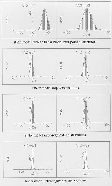
Figure 4a - Distributions as represented by static
and linear segmental models of the first two cepstral coefficients
for the middle state of  .
.
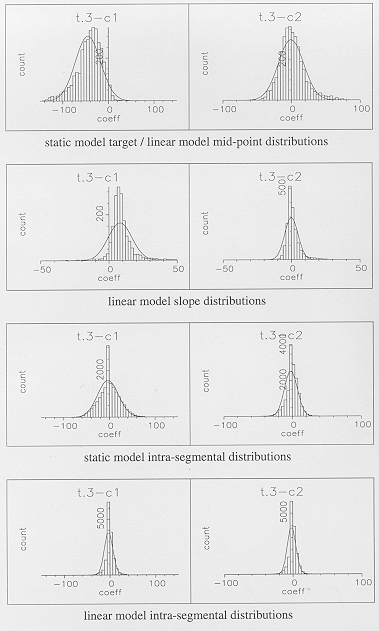
Figure 4b - Distributions as represented by static and linear segmental models of the first two cepstral coefficients for the final state of / t/.
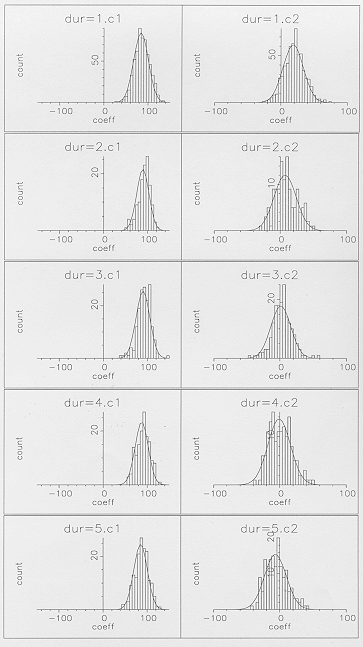
Figure 5 - Target/mid-point distributions of the
first two cepstral coefficients for the middle state of  ,
plotted for individual segment durations of 1 to 5 frames.
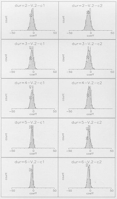
Figure 6a - Linear model slope distributions of
the first two cepstral coefficients for the middle state of  ,
plotted for individual segment durations of 2 to 6 frames.
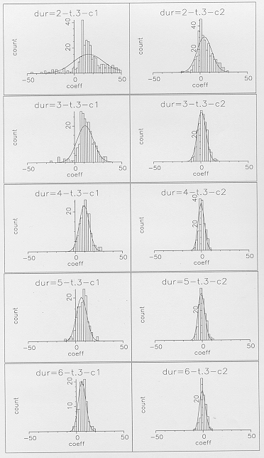
Figure 6b - Linear model slope distributions of
the first two cepstral coefficients for the final state of  ,
plotted for individual segment durations of 2 to 6 frames.
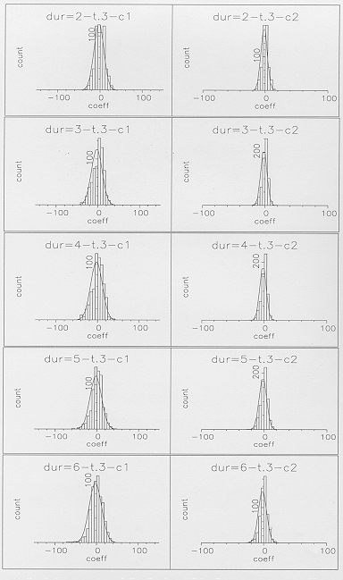
Figure 7 - Static intra-segmental distributions
of the first two cepstral coefficients for the final state of
 , plotted for individual segment durations of 2 to 6 frames.
Acknowledgements
The author would like to thank both Dr. Mark Huckvale at UCL and
Dr. Martin Russell at SRU for their help and advice on the work
which forms the subject of this paper.
Digalakis, V. (1992) Segment-based stochastic models of spectral dynamics for continuous speech recognition, PhD Thesis, Boston University.
Holmes, W.J. and Huckvale, M. (1994) "Why have HMMs been so successful for automatic speech recognition and how might they be improved?", Speech, Hearing and Language, UCL Work in Progress, Vol. 8, 207-219.
Holmes, W.J and Russell, M.J (1995a) Experimental evaluation of segmental HMMs, Proc. IEEE ICASSP, Detroit, 536-539.
Holmes, W.J. and Russell, M.J. (1995b) Speech recognition using a linear dynamic segmental HMM, Proc. EUROSPEECH'95, Madrid, 1611-1614.
Holmes, W.J and Russell, M.J. (1996) Modeling speech variability with segmental HMMs, Proc. IEEE ICASSP, Atlanta, 447-450.
Ostendorf, M., Digalakis, D. and Kimball, O.A. (1996) From HMMs to Segment Models: A Unified View of Stochastic Modeling for Speech Recognition, IEEE Trans. SAP, to be published.
Russell, M.J. (1993) A segmental HMM for speech pattern modelling,
Proc. IEEE ICASSP, Minneapolis, 499-502.
© 1996 Wendy J. Holmes
 Back to SHL 9 Contents
 Back to Phonetics and Linguistics Home Page