Speech Filing System
How To: Phonetic Analysis using Formant Measurements
This document provides a tutorial introduction to the use of SFS for the analysis of the phonetic properties of speech based on measurements of formant frequencies. The tutorial demonstrates how to annotate the signal, how to perform formant analysis, how to extract formant frequencies and how to analyse the resulting data sets. This tutorial refers to versions 4.6 and later of SFS.
Contents
- Formant analysis strategy
- Acquiring and annotating the audio signal
- Formant analysis
- Finding average formant frequencies
- Data analysis
1. Formant Analysis Strategy
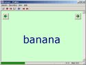
Perhaps the most obvious way to do formant analysis with SFS is to just load up an audio signal, choose Tools|Speech|Display|Cross-section, then make measurements of formant frequencies interactively, writing the results down on a piece of paper, see figure 1.1. You can then type your results into a statistics package and make whatever comparisons you need. This is not the strategy we will be presenting in this tutorial.
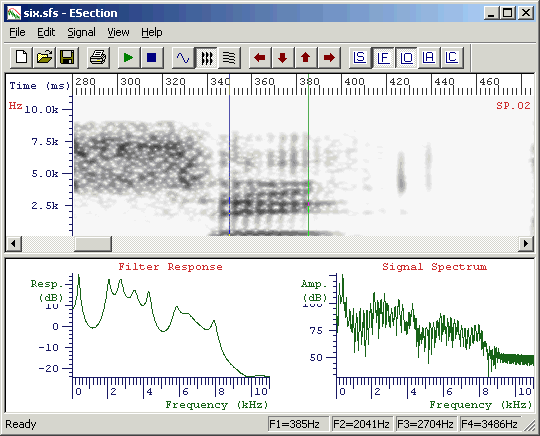
Figure 1.1 - Interactive formant measurement (frequencies in status bar)
There are a number of deficiencies in the direct, interactive route:
- Lack of consistency: how do you know that you are positioning the cursors in a consistent fashion across many instances?
- Potential bias: are you sure you haven't chosen the position of the cursors to obtain the expected formant frequency values?
- Inflexibility: if you want to go back and change the way the formants are measured, or if you want to go back and collect other data (e.g. durations), you have to go through all the data again without knowing exactly how you made the first set of measurements.
- Cost: measuring interactively is slow and expensive on time. If you can use a speech corpus that has been phonetically labelled, then you can be much more productive by exploiting those labels.
- Amount of data: a semi-automatic procedure can analyse more data and provide a wider range of statistics on the distribution of formant frequencies.
The strategy we will be presenting in this tutorial follows these steps:
- Acquire and annotate the signal
- Perform automatic formant analysis on all the speech data
- Use a script to extract the distribution of formant values within and across segments
- Analyse the distributions of formant frequencies
2. Acquiring and Annotating the audio signal
Acquiring the signal
You can use the SFSWin program to record directly from the audio input on your computer. Only do this if you know that your audio input is of good quality, since many PCs have rather poor quality audio. In particular, microphone inputs on PCs are commonly very noisy.
To acquire a signal using SFSWin, choose File|New, then Item|Record. See Figure 2.1. Choose a suitable
sampling rate, at least 16000 samples/sec is recommended. It is usually not necessary to choose a rate faster than 22050 samples/sec for speech signals.
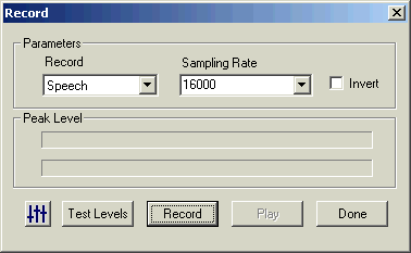
Figure 2.1 - SFSWin record dialog
If you choose to acquire your recording into a file using some other program, or if it is already in an audio file, choose Item|Import|Speech rather than Item|Record to load the recording into SFS. If the file is recorded in plain PCM format in a WAV audio file, you can also just open the file with File|Open. In this case, you will be offered a choice to "Copy contents" or "Link to file" to the WAV file. See Figure 2.2. If you choose copy, then the contents of the audio recording are copied into the SFS file. If you choose link, then the SFS file simply "points" to the WAV file so that it may be processed by SFS programs, but it is not copied (this means that if the WAV file is deleted or moved SFS will report an error).
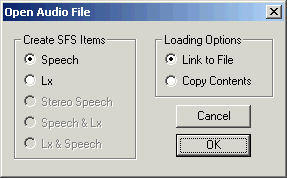
Figure 2.2 - SFSWin open WAV file dialog
Preparing the signal
If the audio recording has significant amounts of background noise, you may like to try and clean the recording using Tools|Speech|Process|Signal enhancement. See Figure 2.3. The default setting is "100% spectral subtraction"; this subtracts 100% of the quietest spectral slice from every frame. This is a fairly conservative level of enhancement, and you can try values greater than 100% to get a more aggressive enhancement, but at the risk of introducing artifacts.
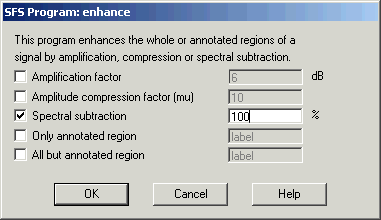
Figure 2.3 - SFSWin enhancement dialog
It is also suggested at this stage that you standardise the level of the recording. You can do this with Tools|Speech|Process|Waveform preparation, choosing the option "Automatic gain control (16-bit)".
Annotating the signal
If you are lucky you will find ready-annotated material suitable for your purposes. Phonetically-annotated speech corpora are becoming more common. If you are thinking of analysing one of the major languages of the world you should investigate whether annotated recordings are available. Often these are supplied to speech researchers at a much lower price than they are made available to speech technology companies. The two major world suppliers of speech corpora are the Linguistic Data Consortium (www.ldc.upenn.edu) and the European Language Resources Association (www.elra.info).
We won't concern ourselves here with converting corpus data to be compatible with SFS, but there exist tools in SFS (such as cnv2sfs and anload) to help make this easier.
Instead we will briefly discuss the use of SFS to add annotations to the signal. We assume that we will only be annotating the regions of the signal where we want to make formant measurements, rather than performing an aligned phonetic annotation of the whole signal (see sister tutorial on Phonetic annotation).
Typically formant measurements are made on syllabic nuclei, where there is likely to be voicing and a relatively unobstructed vocal tract. We'll describe the annotation of monophthongal vowels, although the procedure could easily be adapted to deal with more complex elements.
From within SFSWin, select the speech item to annotate and choose Tools|Speech|Annotate|Manually. Enter a suitable name for the annotations (say, "labels"). The speech signal will be displayed, with a box at the bottom of the display where the annotations may be added/edited. Adjust the display to show waveforms and/or spectrograms as you wish. Use the cursors to isolate regions of the signal until you find the first vowel segment you want to annotate. Zoom in so that the vowel region is clearly visible - perhaps filling about one-quarter of the display. See Figure 2.4.
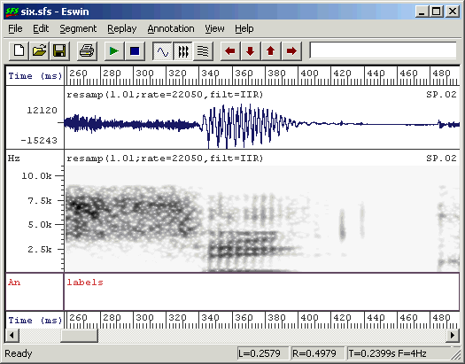
Figure 2.4 - Ready for annotation
The next question is how best to position the annotations? Should one attempt to determine the "centre" of the vowel, or its "edges", or where the formants are "stationary"? The problem is that none of these have clear, unambiguous definitions. The best choice is the one that makes the least assumptions and has the least potential for bias. I suggest choosing a strategy for labelling that is easy and repeatable. In the case of Figure 2.4, where the vowel is preceded and followed by a voiceless consonant, then the labels should go at the start and end of voicing. In circumstances where the voiced region is shared with another voiced segment, consider estimating the point which is acoustically half-way between the segments. It is then reasonable to propose that one segment dominates on one side of the label, while the other segment dominates on the other side. Once the labels are positioned we can try various programmed strategies for reliably extracting formant frequencies from the region.
To add an annotation, position the left cursor at the start of the region to annotate, and the right cursor at the end. Then using the keyboard, type the following:
[A] [label] [RETURN]

[B] [/] [RETURN]
The [A] key is a keyboard shortcut meaning label the left cursor, the [B] key is a keyboard shortcut meaning label the right cursor. In Figure 2.5 we have labelled a segment as being "I_six", that is the vowel /I/ in the word "six". We have marked the end of the segment with "/".
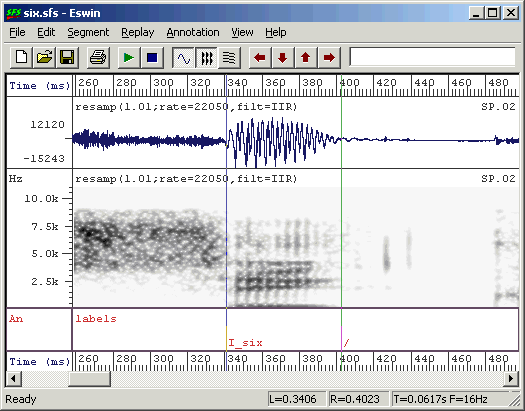
Figure 2.5 - Annotated vowel segment
The decision about how to label the regions will depend on the kind of phonetic analysis you are planning to undertake. Since adding information to the label is easy when you are doing the labelling and very difficult to do retrospectively, consider labelling with information about the context as well as the identity of the segment. You may find in your analysis that your assumptions about allophonic variation are wrong, and that identically-labelled segments actually belong to different phonological categories!
One final useful piece of advice is to fill in information about the identity of the speaker and the recording session in the SFS file header. This information may be useful in allowing us to find files and label graphs later. To do this, select option File|Properties in SFSWin and complete the form shown in Figure 2.6.
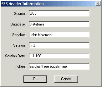
Figure 2.6 - SFSWin File properties
3. Formant Analysis
Introduction
It is worth mentioning at this point that formant analysis is not an exact science. The task the computer is trying to do is estimate the natural frequency of vocal tract resonances given a short section of speech signal picked up by a microphone. The task is made complex because the only way information about the resonances gets into the microphone signal is if the resonances are excited with sounds generated elsewhere in the vocal tract - typically from the larynx. Thus the program has to make assumptions about the nature of this source signal to determine how that signal has been modified by the vocal tract resonances. It may be the case that peaks in the spectrum of the sound are caused by vocal tract resonances, but they may be properties of the source. Likewise, it may be the case that every formant is excited, but it may be that the source simply had no energy at a resonant frequency and it was not excited.
In addition formant analysis is made difficult by the fact that the articulators are constantly moving and the source is changing while producing speech, that the sound signal generated by the vocal tract is possibly contaminated by noise and reverberation before it enters the microphone, and that sometimes formants can get very close together in frequency - so that two resonances can give rise to a single spectral peak. All this without even mentioning the problems that arise at high fundamental frequencies, when formant estimates are likely to biased towards the nearest harmonic frequency.
In all, we should expect that our formant analysis will give rise to "errors", and rather than ignoring them, or hoping they have no effect, we should build in the possibility of measurement error into our procedures.
Fixed frame analysis
The most common means to obtain formant frequency measurements from a speech signal is through linear prediction on short fixed-length sections (frames) of the signal - typically 20-30ms windows. These windows are stepped by 10ms to give spectral peak estimates 100 times per second of signal. Typically each frame delivers about 6 spectral peaks from a signal sampled at 10,000 samples/sec. Not all these peaks are caused by formants, and so a post-processing stage is required to label some of the peaks as being caused by "F1", "F2", etc. This post-processing stage usually makes assumptions about the typical frequency and bandwidth range of vocal tract resonances and their rate of change.
The currently best program in SFS to perform fixed-frame formant analysis is the formanal program. This can be found in SFSWin under Tools|Speech|Analysis|Formant estimates track. The formant analysis code in this program was originally written by David Talkin and John Shore as part of the Entropic Signal Processing System and is used under licence from Microsoft. The current SFS implementation does not have any user-changeable signal processing parameters, see Figure 3.1.
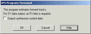
Figure 3.1 - SFSWin Formant estimates dialog
The formanal program performs these processing steps:
- Downsamples the signal to 10,000 samples/sec
- High-pass filters at 75Hz
- Pre-emphasises the signal
- Performs linear prediction by autocorrelation on 50ms windows
- Root solves the linear prediction polynomial to obtain spectral peaks
- Finds the best assignment of peaks to formants over each voiced region of the signal using a dynamic programming algorithm.
Example output is shown in Figure 3.2.
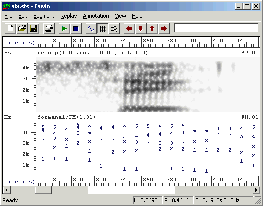
Figure 3.2 - Example of formant estimation output
Pitch-synchronous analysis
Fixed-frame analysis works well in many situations, and you should certainly try the formanal program on your recordings before attempting anything more sophisticated.
However with its large windows and DP tracking formanal will tend to produce rather smooth formant contours which may not reflect accurately the moment-to-moment changes of the vocal tract. A potentially more exact means of obtaining formant frequency measurements is to analyse the data pitch-synchronously. Pitch synchronous formant analysis divides the signal up into windows according to a set of pitch epoch markers, such that each analysis window is simply one pitch period long. The result is a set of formant estimates that are output at a rate of one frame per pitch period rather than one frame per 10ms. There are other technical reasons why we expect individual pitch periods as being a better basis for formant estimation.
To perform pitch-synchronous formant analysis, we can use the SFS fmanal program. This program is less sophisticated than formanal and we have to do some careful preparation of the signal before running it. In particular we need to downsample the signal to about 10,000 samples/sec and we need to generate a set of pitch epoch markers. We'll discuss these in turn:
- Downsampling
- If the signal is sampled at a rate higher than about 12,000 samples/sec, I suggest that you first downsample the signal to about 10,000 samples/sec. Downsampling puts more weight on the peaks below 5kHz which are most important perceptually. To do this, select the signal in SFSWin and choose Tools|Speech|Process|Resample, see Figure 3.3. Put in a sampling rate of 10,000 samples/sec (or if the original signal is at 22050 or 44100 samples/sec, put in 11025 samples/sec).
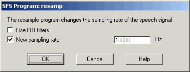
Figure 3.3 - SFSWin resampling dialog - Pitch epoch marking if Laryngograph signal available
- The most reliable way to obtain pitch epoch markers is to make a Laryngograph recording at the same time as the speech signal is recorded. The Laryngograph (www.laryngograph.com) is a specialist piece of equipment that uses two neck electrodes to monitor vocal fold contact area. The resulting stereo signal can be recorded directly into SFSWin or imported from a file using Item|Import|Lx.
From the Laryngograph signal, a set of pitch epoch markers (Tx) can be found from Tools|Lx|Pitch period estimation.
- Pitch epoch marking without a Laryngograph signal
- A less reliable means to get pitch epoch markers is to analyse the speech signal for periodicity. This can work well for clean, non-reverberant audio signals. To do this, select the speech signal in SFSWin and choose Tools|Speech|Analysis|Fundamental frequency|Pitch epoch location and track, see Figure 3.4.
Figure 3.4 - SFSWin pitch epoch track dialog
The result of the preparation should be two items in the SFS file: a downsampled speech signal and a set of pitch epoch markers (Tx). To perform pitch-synchronous formant analysis, select these two items and choose Tools|Speech|Analysis|Formants estimation. Then select the option "Use Tx for pitch synchronous at offset", leaving the offset value as the default of 0. See Figure 3.5.
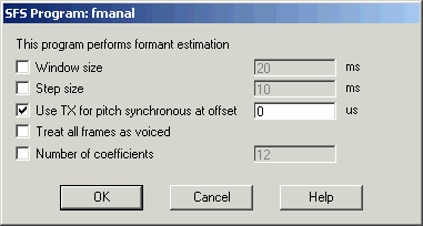
Figure 3.5 - SFSWin pitch-synchronous formant analysis dialog
An example of pitch synchronous formant analysis is shown in Figure 3.6. You can see that the formant frames now occur once per pitch period rather than once per 10ms.
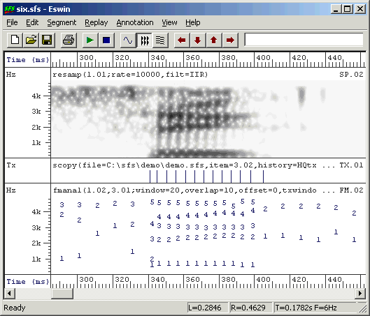
Figure 3.6 - Example of pitch-synchronous formant estimation output
4. Finding average formant frequencies
We are now in a position to find average formant frequencies in our data. There are three types of average we could consider: (i) the average within a vowel segment, (ii) the average over all segments of a given type for one speaker, or (iii) the average over all vowel segments of a given type spoken by multiple speakers. We'll look at these in turn.
Average within a segment
We have annotated our speech signal with labels identifying the vocalic regions where we would like to make a single formant frequency measurement. However, within that region the formant analysis program may have delivered a number of frames of formant estimates. Also the region may cover the whole vocalic segment while we are interested in a single value which "characterises" the vowel. Thus we need to decide how to calculate a characteristic value from some part of the annotated region. In the process we need to take into account the typical contextual changes that occur to vowel formant frequencies in syllables and the typical errors made by formant frequency estimation techniques.
Method 1. Mean over whole segment
We'll start with the most obvious: taking a mean over the whole segment. To demonstrate this, we'll write a script to extract the mean F1, F2 and F3 of each annotated region and save these to a text file in "comma-separated value" (CSV) format. This script is written in the SFS Speech Measurement Language (SML). The script is as follows:
/* fmsummary.sml - summarise formant measurements from labels */

/* get mean formant value for a segment */
function var measure_mean(stime,etime,pno)
{
    var    stime;    /* start time */
    var    etime;    /* end time */
    var    pno;    /* FM parameter # */
    var    t;        /* time */
    var    sum;    /* sum of values */
    var    cnt;    /* # values */

    /* calculate mean over whole segment */
    sum=0;
    cnt=0;
    t=next(FM,stime);
    while (t < etime) {
        sum = sum + fm(pno,t);
        cnt = cnt + 1;
        t = next(FM,t);
    }

    return(sum/cnt);
}

/* for each file to be processed */
main {
    var    num;    /* # annotated regions */
    var    i;
    var stime,etime;
    var    vf1,vf2,vf3;

    num = numberof(".");
    /* for each annotation */
    for (i=1;i<=num;i=i+1) if (compare(matchn(".",i),"/")!=0) {
        stime = timen(".",i);
        etime = stime + lengthn(".",i);
        vf1 = measure_mean(stime,etime,5);
        vf2 = measure_mean(stime,etime,8);
        vf3 = measure_mean(stime,etime,11);
        /* output in CSV format */
        print "\"",$filename,"\",\"",matchn(".",i),"\","
        print vf1,",",vf2,",",vf3,"\n"
    }
}
|
This script calls a function measure_mean() for each annotated region for each formant parameter. The script assumes that there is already a FORMANT item in the file, which can be either fixed-frame or pitch synchronous. To run this script, select the annotation item and the formant item to be processed and choose menu option Tools|Run SML script. Enter the file containing the script above and the name of a text file to recive the output, see Figure 4.1.
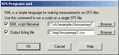
Figure 4.1 - SFSWin run SML script dialog
The result of running this script looks like this:
"C:\data\ABI\short\brm_f_01_01.sfs","sil", 1120.2540, 2913.2937, 4104.5054 "C:\data\ABI\short\brm_f_01_01.sfs","k", 1146.8917, 2651.2722, 3779.6567 "C:\data\ABI\short\brm_f_01_01.sfs","ae", 789.7859, 1805.1616, 2465.6825 "C:\data\ABI\short\brm_f_01_01.sfs","ng", 662.5625, 1246.0687, 2189.2784 "C:\data\ABI\short\brm_f_01_01.sfs","g", 395.1142, 918.3024, 2061.2703 "C:\data\ABI\short\brm_f_01_01.sfs","ax", 375.5445, 1579.8998, 2311.1436 "C:\data\ABI\short\brm_f_01_01.sfs","r", 438.3379, 1350.3599, 2410.2007 "C:\data\ABI\short\brm_f_01_01.sfs","uw", 462.2808, 1760.6830, 2486.4146 ... |
This CSV format is convenient to use because many spreadsheet and statistics packages can read data in this format. Figure 4.2 shows these data loaded into Excel.
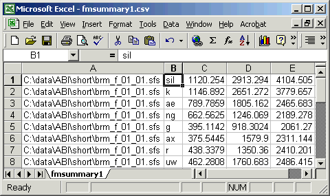
Figure 4.2 - Formant data loaded into Excel
Method 2. Mean over middle third of segment
Since we expect formant values at the edges of the segment to be less characteristic of the segment than values towards the middle, a refinement of method 1 would be to restrict the analysis to the central third of the segment in time. Here is a replacement measurement function for the script above:
/* get mean formant value for a segment */
function var measure_mean_third(stime,etime,pno)
{
    var    stime;    /* start time */
    var    etime;    /* end time */
    var    pno;    /* FM parameter # */
    var    t;        /* time */
    var    sum;    /* sum of values */
    var    cnt;    /* # values */
    var    len;

    /* adjust times to central third */
    len = etime - stime;
    stime = stime + len/3;
    etime = etime - len/3;

    /* calculate mean */
    sum=0;
    cnt=0;
    t=next(FM,stime);
    while (t < etime) {
        sum = sum + fm(pno,t);
        cnt = cnt + 1;
        t = next(FM,t);
    }

    return(sum/cnt);
}
|
Method 3. Median over whole segment
The disadvantage of the mean is that we know that formant tracking errors can occasionally produce wildly inaccurate frequency values. For example, a common tracking error is to relabel F1 as F2, and F2 as F3, and so on. It would seem to be a good idea to remove from the calculation any outlier values. One easy way to do this is to calculate the median over the segment rather than the mean. Here is the adjustment to our script:
/* calculate a median */
function var median(table,len)
{
    var table[];    /* array of values */
    var len;        /* # values */
    var    i,j,tmp;

    /* sort table */
    for (i=2;i<=len;i=i+1) {
        j = i;
        tmp = table[j];
        while (table[j-1] > tmp) {
            table[j] = table[j-1];
            j = j - 1;
            if (j==1) break;
        }
        table[j] = tmp;
    }

    /* return middle value */
    if ((len%2)==1) {
        return(table[1+len/2])
    }
    else {
        return((table[len/2]+table[1+len/2])/2);
    }
}

/* get median formant value for a segment */
function var measure_median(stime,etime,pno)
{
    var    stime;    /* start time */
    var    etime;    /* end time */
    var    pno;    /* FM parameter # */
    var    t;        /* time */
    var af[1:1000];    /* array of values */
    var    nf;        /* # values */

    /* calculate median */
    nf=0;
    t=next(FM,stime);
    while ((t < etime)&&(nf < 1000)) {
        nf = nf+1;
        af[nf] = fm(pno,t);
        t = next(FM,t);
    }

    return(median(af,nf));
}
|
Method 4. Trimmed mean over whole segment
The disadvantage of the median is that it only picks one value as representative of the formant contour for the segment. One way to get a smoothed estimate but disregard outliers is to use the "trimmed mean" - this is just the mean of the values at the middle of the distribution. In the following variation we calculate a trimmed mean of the central 60% (disregarding the lowest 20% and the highest 20%) - but adjust as you see fit.
/* calculate trimmed mean */
function var trimmean(table,len)
{
    var table[];    /* array of values */
    var len;        /* # values */
    var    i,j,tmp;
    var    lo,hi;

    /* sort table */
    for (i=2;i<=len;i=i+1) {
        j = i;
        tmp = table[j];
        while (table[j-1] > tmp) {
            table[j] = table[j-1];
            j = j - 1;
            if (j==1) break;
        }
        table[j] = tmp;
    }

    /* find mean over middle portion */
    lo = trunc(0.5 + 1 + len/5);    /* lose bottom 20% */
    hi = trunc(0.5 + len - len/5);    /* lose top 20% */
    j=0;
    tmp=0;
    for (i=lo;i<=hi;i=i+1) {
        tmp = tmp + table[i];
        j = j + 1;
    }
    return(tmp/j);
}

/* get median formant value for a segment */
function var measure_trimmed_mean(stime,etime,pno)
{
    var    stime;    /* start time */
    var    etime;    /* end time */
    var    pno;    /* FM parameter # */
    var    t;        /* time */
    var af[1:1000];    /* array of values */
    var    nf;        /* # values */

    /* collect values */
    nf=0;
    t=next(FM,stime);
    while ((t < etime)&&(nf < 1000)) {
        nf = nf+1;
        af[nf] = fm(pno,t);
        t = next(FM,t);
    }

    return(trimmean(af,nf));
}
|
Method 5. Find straight line of best fit
Since we don't expect the formant frequency to be constant over the segment, another approach is to fit a line to the formant values and choose the value of that line at the centre point of the segment as representative of the segment as a whole. To fit a line, we perform a least-squares procedure as follows:
/* calculate last-squares fit and return value at time */
function var lsqfit(at,af,nf,t)
{
    var    at[];    /* array of times */
    var    af[];    /* array of frequencies */
    var    nf;        /* # values */
    var    t;        /* output time */
    var    i
    stat x,y,xy
    var    a,b;    /* coefficients */

    /* collect parameters */
    for (i=1;i<=nf;i=i+1) {
        x += at[i];
        y += af[i]
        xy += at[i]*af[i]
    }

    /* find coefficients of line */
    b = (nf*xy.sum-x.sum*y.sum)/(nf*x.sumsq-x.sum*x.sum);
    a = (y.sum - b*x.sum)/nf;

    return(a + b*t);
}

/* get mid point of formant trajectory for a segment */
function var measure_linear(stime,etime,pno)
{
    var    stime;    /* start time */
    var    etime;    /* end time */
    var    pno;    /* FM parameter # */
    var    t;        /* time */
    var at[1:1000];    /* array of time */
    var af[1:1000];    /* array of values */
    var    nf;        /* # values */

    /* collect values */
    nf=0;
    t=next(FM,stime);
    while ((t < etime)&&(nf < 1000)) {
        nf = nf+1;
        at[nf] = t;
        af[nf] = fm(pno,t);
        t = next(FM,t);
    }

    return(lsqfit(at,af,nf,(stime+etime)/2));
}
|
Method 6. Find quadratic of best fit
Finally, we refine the last approach by fitting a quadratic rather than a straight line to the formant values. This accommodates the fact that formant trajectories are often curved through a segment. A possible disadvantage is that we may become over sensitive to outliers. Here are the modifications needed:
/* calculate last-squares fit of quadratic and return value at time */
function var quadfit(at,af,nf,t)
{
    var    at[];    /* array of times */
    var    af[];    /* array of frequencies */
    var    nf;        /* # values */
    var    t;        /* output time */
    var    i;
    var    a,b,c;    /* coefficients */
    var    mat1[1:4];    /* normal matrix row 1 */
    var    mat2[1:4];    /* normal matrix row 2 */
    var    mat3[1:4];    /* normal matrix row 3 */

    /* collect parameters */
    for (i=1;i<=nf;i=i+1) {
        mat1[1] = mat1[1] + 1;
        mat1[2] = mat1[2] + at[i];
        mat1[3] = mat1[3] + at[i] * at[i];
        mat1[4] = mat1[4] + af[i];
        mat2[1] = mat2[1] + at[i];
        mat2[2] = mat2[2] + at[i] * at[i];
        mat2[3] = mat2[3] + at[i] * at[i] * at[i];
        mat2[4] = mat2[4] + at[i] * af[i];
        mat3[1] = mat3[1] + at[i] * at[i];
        mat3[2] = mat3[2] + at[i] * at[i] * at[i];
        mat3[3] = mat3[3] + at[i] * at[i] * at[i] * at[i];
        mat3[4] = mat3[4] + at[i] * at[i] * af[i];
    }

    /* reduce lines 2 and 3, column 1 */
    for (i=4;i>=1;i=i-1) {
        mat2[i] = mat2[i] - mat1[i]*mat2[1]/mat1[1];
        mat3[i] = mat3[i] - mat1[i]*mat3[1]/mat1[1];
    }

    /* reduce line 3 column 2 */
    for (i=4;i>=2;i=i-1) {
        mat3[i] = mat3[i] - mat2[i]*mat3[2]/mat2[2];
    }

    /* calculate c */
    c = mat3[4]/mat3[3];

    /* back substitute to get b */
    b = (mat2[4] - mat2[3]*c)/mat2[2];

    /* back substitute to get a */
    a = (mat1[4] - mat1[3]*c - mat1[2]*b)/mat1[1];

    return(a + b*t + c*t*t);
}

/* get mid point of formant trajectory for a segment */
function var measure_quadratic(stime,etime,pno)
{
    var    stime;    /* start time */
    var    etime;    /* end time */
    var    pno;    /* FM parameter # */
    var    t;        /* time */
    var at[1:1000];    /* array of time */
    var af[1:1000];    /* array of values */
    var    nf;        /* # values */

    /* collect values */
    nf=0;
    t=next(FM,stime);
    while ((t < etime)&&(nf < 1000)) {
        nf = nf+1;
        at[nf] = t;
        af[nf] = fm(pno,t);
        t = next(FM,t);
    }

    return(quadfit(at,af,nf,(stime+etime)/2));
}
|
In the next section we'll apply these approaches to the study of the distribution of formant values for a particular segment type for a single speaker, and investigate which gives us the least variable results.
Average within a speaker
So far we have shown a number of ways in which to extract a characteristic formant frequency value from each annotated region of the signal. In this section we will look at the distribution of those values for a number of instances of a single type of annotated region for a single speaker. This will not only demonstrate how to collect data across a number of files, but it will also allow us to make a simple empirical study of the performance of the six different methods.
The script below calls the measure_mean() function on all instances of a given labelled region found in the input files. It then collects the values into a histogram and plots the histogram and a modelled normal distribution for each formant. It also reports the mean and standard deviation of the estimated characteristic formant frequencies for the segment.
/* fmplot1.sml -- plot distribution of formant frequency averages */
/* - uses mean over whole annotated region */

stat    f1;            /* f1 distribution */
stat    f2;            /* f2 distribution */
stat    f3;            /* f3 distribution */
var        hf1[0:100];    /* f1 histogram (50Hz bins) */
var        hf2[0:100];    /* f2 histogram (50Hz bins) */
var        hf3[0:100];    /* f3 histogram (50Hz bins) */

string    label;    /* annotation label to measure */
file    gop;    /* graphics output */

/* get mean formant value for a segment */
function var measure_mean(stime,etime,pno)
{
    var    stime;    /* start time */
    var    etime;    /* end time */
    var    pno;    /* FM parameter # */
    var    t;        /* time */
    var    sum;    /* sum of values */
    var    cnt;    /* # values */

    /* calculate mean over whole segment */
    sum=0;
    cnt=0;
    t=next(FM,stime);
    while (t < etime) {
        sum = sum + fm(pno,t);
        cnt = cnt + 1;
        t = next(FM,t);
    }

    if (cnt > 0) return(sum/cnt) else return(ERROR);
}

/* normal distribution */
function var normal(st,x)
stat st;
{
    var x;
    x = x - st.mean;
    return(exp(-0.5*x*x/st.variance)/sqrt(2*3.14159*st.variance));
}

/* plot histogram overlaid with normal distribution */
function var plotdist(st,hs)
stat st;
var hs[];
{
    var    i;
    var    xdata[1:2];
    var ydata[0:4000];

    /* set up x-axes */
    xdata[1]=0;
    xdata[2]=4000;
    plotxdata(xdata,1)

    /* plot histogram */
    plotparam("type=hist");
    for (i=0;i<=80;i=i+1) ydata[i] = hs[i]/st.count;
    plot(gop,1,ydata,81);

    /* plot normal distribution */
    plotparam("type=line");
    for (i=0;i<4000;i=i+1) ydata[i]=50*normal(st,i);
    plot(gop,1,ydata,4000);
}

/* record details of a single segment */
function var recordsegment(stime,etime,pno,st,hs)
stat st;
var hs[];
{
    var stime,etime,pno;
    var f

    f = measure_mean(stime,etime,pno);
    if (f) {
        st += f;
        hs[trunc(f/50)] = hs[trunc(f/50)] + 1;
    }
}

/* initialise */
init {
    string ans

    /* get label */
    print#stderr "Enter label to find : ";
    input label;

    /* where to send graphs */
    print#stderr "Send graph to file 'dig.gif' ? (Y/N) "
    input ans
    if (index("^[yY]",ans)) {
        openout(gop,"|dig -g -s 500x375 -o dig.gif");
    } else openout(gop,"|dig");
}

/* for each file to be processed */
main {
    var        i,num,stime,etime

    num=numberof(label);
    print#stderr "File ",$filename," has ",num," matching annotations\n";

    for (i=1;i<=num;i=i+1) {
        stime = next(FM,timen(label,i));
        etime = timen(label,i) + lengthn(label,i);
        recordsegment(stime,etime,5,f1,hf1);    /* 5 = F1 */
        recordsegment(stime,etime,8,f2,hf2);    /* 8 = F2 */
        recordsegment(stime,etime,11,f3,hf3);    /* 11 = F3 */
    }
}

/* display summary statistics and graphs */
summary {
    print#stderr "F1 = ",f1.mean," +/-",f1.stddev,"Hz (",f1.count:1,")\n";
    print#stderr "F2 = ",f2.mean," +/-",f2.stddev,"Hz (",f2.count:1,")\n";
    print#stderr "F3 = ",f3.mean," +/-",f3.stddev,"Hz (",f3.count:1,")\n";

    plottitle(gop,"/"++label++"/ formant distributions 1");
    plotparam("title=(mean over whole segment)");
    plotparam("xtitle=Frequency (Hz)");
    plotparam("ytitle=Probability");

    if (f1.variance > 0) plotdist(f1,hf1);
    if (f2.variance > 0) plotdist(f2,hf2);
    if (f3.variance > 0) plotdist(f3,hf3);
}
|
We will run this script over 150 phonetically annotated sentences from one speaker that form part of the SCRIBE corpus. We'll just look at the distribution of the formant frequencies among 65 instances of /A:/ in those sentences. Because this script processes multiple files and accepts user input, it must be run from the command line, not from within SFS. This presupposes that the SFS installation program directory is on the search path for the command line tool. The command line tool can be found in the Windows Start|Programs menu: sometimes it can be found under Start|Programs|Accessories|Command Prompt, sometimes under Start|Programs|Accessories|System Tools|Command Prompt. To check the command-line path, type PATH in response to the prompt:
C:\Documents and Settings\Mark> PATH
If SFS is installed correctly, you should see "C:\Program Files\SFS\Program" on the list of directories searched by the command line tool. If it is not there, look at the installation instructions for SFS - found under Start|Programs|Speech Filing System|SFS Installation Notes. To run our script we need to enter a command patterned after:
C:\Program Files\SFS\Examples> sml script.sml filelist
Figure 4.3 shows what this would look like within the command line tool window.
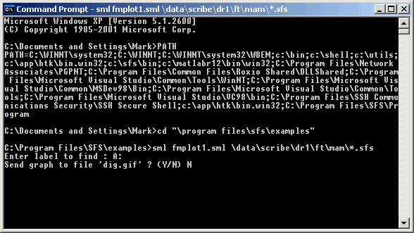
Figure 4.3 - Command line execution of SML script
The graphical output of the script is shown in Figure 4.4.
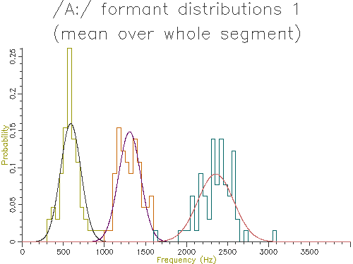
Figure 4.4 - Analysis of 65 /A:/ vowels, method 1
This figure shows quite clearly the breadth of the formant frequency distributions even when all the vowels are from the same speaker. The estimated characteristic formant frequencies for /A:/ for this speaker is also output by the script:
F1 =   579.2066 +/-  112.6763Hz (65)
F2 =  1278.4254 +/-  127.9527Hz (65)
F3 =  2332.7904 +/-  210.0033Hz (65)
Figures 4.5 to 4.9 show the output of similar scripts set up to use each of the other methods described in the last section
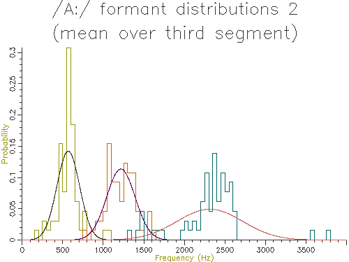
Figure 4.5 - Analysis of 65 /A:/ vowels, method 2
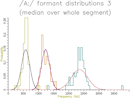
Figure 4.6 - Analysis of 65 /A:/ vowels, method 3
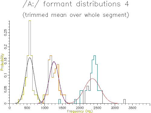
Figure 4.7 - Analysis of 65 /A:/ vowels, method 4
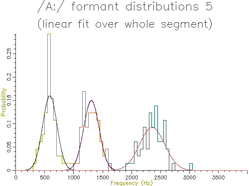
Figure 4.8 - Analysis of 65 /A:/ vowels, method 5
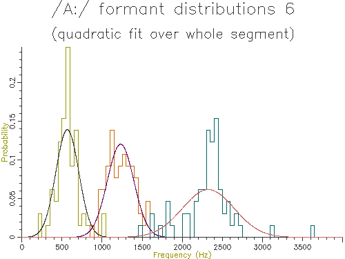
Figure 4.9 - Analysis of 65 /A:/ vowels, method 6
The table below shows the mean and standard deviation of the characteristic formant frequency for each formant for each of the analysis methods:
| Method | F1 | F2 | F3 | |||
|---|---|---|---|---|---|---|
| Mean (Hz) | Dev (Hz) | Mean (Hz) | Dev (Hz) | Mean (Hz) | Dev (Hz) | |
| 1. Mean whole | 588.6 | 125.1 | 1306.2 | 134.3 | 2356.0 | 217.7 |
| 2. Mean third | 567.8 | 140.4 | 1216.6 | 175.6 | 2314.1 | 404.6 |
| 3. Median | 576.9 | 136.9 | 1234.2 | 136.7 | 2357.8 | 272.2 |
| 4. Trimmed mean | 575.3 | 123.4 | 1263.0 | 135.3 | 2357.2 | 227.2 |
| 5. Fit line | 588.2 | 125.0 | 1305.0 | 133.6 | 2355.1 | 217.0 |
| 6. Fit quadratic | 565.9 | 143.3 | 1230.5 | 165.6 | 2324.0 | 323.1 |
Looking at the table, the lowest variance for F1 comes through using the trimmed mean, while the lowest variance for F2 and F3 comes from the straight line fit. Which is the best method? The problem is choosing a method that is robust to the typical errors in formant estimation. The trimmed mean seems a simple and robust measure and has among the lowest variance in our data.
Speaker Normalisation
So far we have looked at collecting formant measurements within a segment and across copies of a segment within one speaker. In this section we look at the problems of collecting formant measurements across speakers. The biggest challenge we face is the standardisation of the range of formant values for each speaker prior to averaging across speakers. Because speakers are of physically different sizes, the absolute value of their formant frequencies will vary because of their size as well as because of any change in accent or style or whatever.
We will only look at a simple means for standardising or normalising formant frequencies. As well as collecting formant measurements from a collection of recordings of a speaker for a single segment type, we will also collect measurements for all related types for the speaker (e.g. over a vowel and over all vowels). We can then represent the characteristic formant frequencies for a segment for a speaker in terms of their relationship to the overall distribution of frequencies for the speaker.
To demonstrate the idea we will first show how to collect segment specific and general measurements for vowels from a number of annotated recordings of a single speaker, delivering a normalised formant estimate. We'll use the trimmed mean to get a characteristic value for each segment.
/* fmnorm.sml - calculate normalised formant measurements for segment */

/* global distribution */
stat    gf1,gf2,gf3;

/* segment specific distribution */
stat    sf1,sf2,sf3;

/* label to find */
string    label;

/* calculate trimmed mean */
function var trimmean(table,len)
{
    var table[];    /* array of values */
    var len;        /* # values */
    var    i,j,tmp;
    var    lo,hi;

    /* sort table */
    for (i=2;i<=len;i=i+1) {
        j = i;
        tmp = table[j];
        while (table[j-1] > tmp) {
            table[j] = table[j-1];
            j = j - 1;
            if (j==1) break;
        }
        table[j] = tmp;
    }

    /* find mean over middle portion */
    lo = trunc(0.5 + 1 + len/5);    /* lose bottom 20% */
    hi = trunc(0.5 + len - len/5);    /* lose top 20% */
    j=0;
    tmp=0;
    for (i=lo;i<=hi;i=i+1) {
        tmp = tmp + table[i];
        j = j + 1;
    }
    if (j > 0) return(tmp/j) else return(ERROR);
}

/* get trimmed mean formant value for a segment */
function var measure_trimmed_mean(stime,etime,pno)
{
    var    stime;    /* start time */
    var    etime;    /* end time */
    var    pno;    /* FM parameter # */
    var    t;        /* time */
    var af[1:1000];    /* array of values */
    var    nf;        /* # values */

    /* calculate trimmed mean */
    nf=0;
    t=next(FM,stime);
    while ((t < etime)&&(nf < 1000)) {
        nf = nf+1;
        af[nf] = fm(pno,t);
        t = next(FM,t);
    }

    return(trimmean(af,nf));
}

/* record details of a single segment */
function var recordsegment(stime,etime,pno,st)
stat st;
{
    var stime,etime,pno;
    var f

    f = measure_trimmed_mean(stime,etime,pno);
    if (f) st += f;
}

/* initialise */
init {
    /* get label */
    print#stderr "Enter label to find : ";
    input label;
}

/* for each file to be processed */
main {
    var    num;    /* # annotated regions */
    var    i;
    var stime,etime;

    num = numberof(".");
    print#stderr "File ",$filename," has ",num," annotations\n";

    /* for each annotation */
    for (i=1;i<=num;i=i+1) {
        stime = timen(".",i);
        etime = stime + lengthn(".",i);
        if (index(label,matchn(".",i))) {
            /* matching label */
            recordsegment(stime,etime,5,sf1);
            recordsegment(stime,etime,8,sf2);
            recordsegment(stime,etime,11,sf3);
        }
        if (index("^[aeiouAEIOU3@QV]",matchn(".",i))) {
            /* some kind of vowel */
            recordsegment(stime,etime,5,gf1);
            recordsegment(stime,etime,8,gf2);
            recordsegment(stime,etime,11,gf3);
        }
    }
}

/* summarise */
summary {
    /* report speaker means */
    print "Speaker means: (",gf1.count:1," segments)\n";
    print "F1 = ",gf1.mean," +/-",gf1.stddev,"Hz\n";
    print "F2 = ",gf2.mean," +/-",gf2.stddev,"Hz\n";
    print "F3 = ",gf3.mean," +/-",gf3.stddev,"Hz\n";

    /* report segment means */
    print "Segment means: (",sf1.count:1," segments)\n";
    print "F1 = ",sf1.mean," +/-",sf1.stddev,"Hz\n";
    print "F2 = ",sf2.mean," +/-",sf2.stddev,"Hz\n";
    print "F3 = ",sf3.mean," +/-",sf3.stddev,"Hz\n";

    /* report normalised means */
    print "Normalised segment means: (",sf1.count:1," segments)\n";
    print "F1 = ",(sf1.mean-gf1.mean)/gf1.stddev," z-score\n";
    print "F2 = ",(sf2.mean-gf2.mean)/gf2.stddev," z-score\n";
    print "F3 = ",(sf3.mean-gf3.mean)/gf3.stddev," z-score\n";
}
|
In this script we collect the mean value of F1, F2 anf F3 for a single segment type, and also collect the mean and variance of F1, F2 and F3 over all vowel segments. We then express F1, F2 and F3 for the given segment as z-scores - positions of the segment mean with respect to the mean and variance of all vowels. The table below shows the output of the script over 200 sentences spoken by one person for two different vowels:
| /A:/ vowel |
|---|
Speaker means: (1847 segments) F1 = 426.0644 +/- 151.5595Hz F2 = 1589.4008 +/- 314.8747Hz F3 = 2496.9879 +/- 239.9074Hz Segment means: (65 segments) F1 = 575.2579 +/- 123.4225Hz F2 = 1263.0107 +/- 135.3098Hz F3 = 2357.1892 +/- 227.2396Hz Normalised segment means: (65 segments) F1 = 0.9844 z-score F2 = -1.0366 z-score F3 = -0.5827 z-score |
| /i:/ vowel |
Speaker means: (1847 segments) F1 = 426.0644 +/- 151.5595Hz F2 = 1589.4008 +/- 314.8747Hz F3 = 2496.9879 +/- 239.9074Hz Segment means: (192 segments) F1 = 336.3615 +/- 83.0778Hz F2 = 1936.3488 +/- 211.8316Hz F3 = 2621.4353 +/- 209.6236Hz Normalised segment means: (192 segments) F1 = -0.5919 z-score F2 = 1.1019 z-score F3 = 0.5187 z-score |
We can now apply this idea to the comparison of formant frequencies across speakers. In this demonstration we will plot the mean F1 and F2 for 5 long monophthongs (/i:/, /u:/, /3:/, /A:/, /O:/) over 10 male and 10 female speakers of a single accent. We'll do this first without normalisation, then with normalisation.
Note: in the data used for this demonstration, speakers can be identified from the fact that the first 8 characters of the filename are specific to the speaker. We will use this to collect the F1 and F2 data on a speaker-dependent basis. Also this database is labelled with ARPABET symbols, not SAMPA.
/* f1f2speaker.sml - F1-F2 diagram for vowels across speakers */

/* list of speakers */
string    stab[1:100];
var    scnt;

/* general vowel distributions */
stat    gf1[1:100];
stat    gf2[1:100];

/* specific vowel distributions */
stat    s1f1[1:100],s1f2[1:100];
stat    s2f1[1:100],s2f2[1:100];
stat    s3f1[1:100],s3f2[1:100];
stat    s4f1[1:100],s4f2[1:100];
stat    s5f1[1:100],s5f2[1:100];

/* output file */
file    gop;

/* function to find speaker code from filename */
function var speakercode(name)
{
    var    code;
    string name;

    name = name:8;    /* first eight characters */
    code = entry(name,stab);
    if (code) return(code);
    scnt=scnt+1;
    stab[scnt]=name;
    return(scnt);
}

/* calculate trimmed mean */
function var trimmean(table,len)
{
    var table[];    /* array of values */
    var len;        /* # values */
    var    i,j,tmp;
    var    lo,hi;

    /* sort table */
    for (i=2;i<=len;i=i+1) {
        j = i;
        tmp = table[j];
        while (table[j-1] > tmp) {
            table[j] = table[j-1];
            j = j - 1;
            if (j==1) break;
        }
        table[j] = tmp;
    }

    /* find mean over middle portion */
    lo = trunc(0.5 + 1 + len/5);    /* lose bottom 20% */
    hi = trunc(0.5 + len - len/5);    /* lose top 20% */
    j=0;
    tmp=0;
    for (i=lo;i<=hi;i=i+1) {
        tmp = tmp + table[i];
        j = j + 1;
    }
    if (j > 0) return(tmp/j) else return(ERROR);
}

/* get trimmed mean formant value for a segment */
function var measure_trimmed_mean(stime,etime,pno)
{
    var    stime;    /* start time */
    var    etime;    /* end time */
    var    pno;    /* FM parameter # */
    var    t;        /* time */
    var af[1:1000];    /* array of values */
    var    nf;        /* # values */

    /* calculate trimmed mean */
    nf=0;
    t=next(FM,stime);
    while ((t < etime)&&(nf < 1000)) {
        nf = nf+1;
        af[nf] = fm(pno,t);
        t = next(FM,t);
    }

    return(trimmean(af,nf));
}

/* record details of a single segment */
function var recordsegment(stime,etime,stf1,stf2)
stat stf1;
stat stf2;
{
    var stime,etime;
    var f

    f = measure_trimmed_mean(stime,etime,5);
    if (f) stf1 += f;
    f = measure_trimmed_mean(stime,etime,8);
    if (f) stf2 += f;
}

/* plot F1-F2 for segment */
function var plotf1f2segment(label,astf1,astf2)
{
    string    label;
    stat    astf1[];
    stat    astf2[];
    var    i;
    var    xdata[1:100];
    var    ydata[1:100];

    /* for each speaker */
    for (i=1;i<=scnt;i=i+1) {
        xdata[i] = astf1[i].mean;
        ydata[i] = astf2[i].mean;
    }
    plotparam("char="++label);

    plotxdata(xdata,0);
    plot(gop,1,ydata,scnt);
}

/* plot F1-F2 graph */
function var plotf1f2()
{
    openout(gop,"|dig");
    plottitle(gop,"Formant variation");
    plotparam("title=no normalisation");
    plotparam("xtitle=F1 Frequency (Hz)");
    plotparam("ytitle=F2 Frequency (Hz)");
    plotparam("type=point");
    plotaxes(gop,1,200,900,1000,2500);

    /* for each segment in turn */
    plotf1f2segment("i",s1f1,s1f2);
    plotf1f2segment("u",s2f1,s2f2);
    plotf1f2segment("3",s3f1,s3f2);
    plotf1f2segment("A",s4f1,s4f2);
    plotf1f2segment("O",s5f1,s5f2);

    close(gop);
}

/* plot F1-F2 for segment */
function var plotf1f2normsegment(label,astf1,astf2)
{
    string    label;
    stat    astf1[];
    stat    astf2[];
    var    i;
    var    xdata[1:100];
    var    ydata[1:100];

    /* for each speaker */
    for (i=1;i<=scnt;i=i+1) {
        xdata[i] = (astf1[i].mean-gf1[i].mean)/gf1[i].stddev;
        ydata[i] = (astf2[i].mean-gf2[i].mean)/gf2[i].stddev;
    }
    plotparam("char="++label);

    plotxdata(xdata,0);
    plot(gop,1,ydata,scnt);
}

/* plot F1-F2 graph */
function var plotf1f2norm()
{
    openout(gop,"|dig");
    plottitle(gop,"Formant variation");
    plotparam("title=with normalisation");
    plotparam("xtitle=F1 Frequency (z-score)");
    plotparam("ytitle=F2 Frequency (z-score)");
    plotparam("type=point");
    plotaxes(gop,1,-1.5,1.5,-2,2);

    /* for each segment in turn */
    plotf1f2normsegment("i",s1f1,s1f2);
    plotf1f2normsegment("u",s2f1,s2f2);
    plotf1f2normsegment("3",s3f1,s3f2);
    plotf1f2normsegment("A",s4f1,s4f2);
    plotf1f2normsegment("O",s5f1,s5f2);

    close(gop);
}

/* for each file to be processed */
main {
    var    num;    /* # annotated regions */
    var    i;
    var stime,etime;
    var    scode;
    string    label;

    /* get code for speaker */
    scode=speakercode($filename);

    /* report file */
    num = numberof(".");
    print#stderr "File ",$filename," has ",num," annotations\n";

    /* for each annotation */
    for (i=1;i<=num;i=i+1) {
        stime = timen(".",i);
        etime = stime + lengthn(".",i);
        label = matchn(".",i);
        switch (label) {    /* ARPABET labels */
        case "iy": recordsegment(stime,etime,s1f1[scode],s1f2[scode]);
        case "uw": recordsegment(stime,etime,s2f1[scode],s2f2[scode]);
        case "er": recordsegment(stime,etime,s3f1[scode],s3f2[scode]);
        case "aa": recordsegment(stime,etime,s4f1[scode],s4f2[scode]);
        case "ao": recordsegment(stime,etime,s5f1[scode],s5f2[scode]);
        }
        if (index("^[aeiou]",label)) {
            /* some kind of vowel */
            recordsegment(stime,etime,gf1[scode],gf2[scode]);
        }
    }
}

/* summarise collected data */
summary {
    /* plot graph unnormalised */
    plotf1f2();

    /* plot graph normalised */
    plotf1f2norm();
}
|
The outputs of the script on 10 male and 10 female speakers are shown in Figures 4.10 and 4.11. The normalised results show considerably less variation across speakers and also less overlap across segment types. In the next section we will look at how we can perform statistical comparisons on these kind of data across speakers and types.
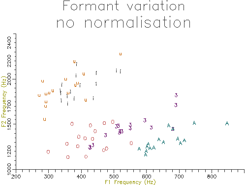
Figure 4.10 - Vowel analysis without normalisation
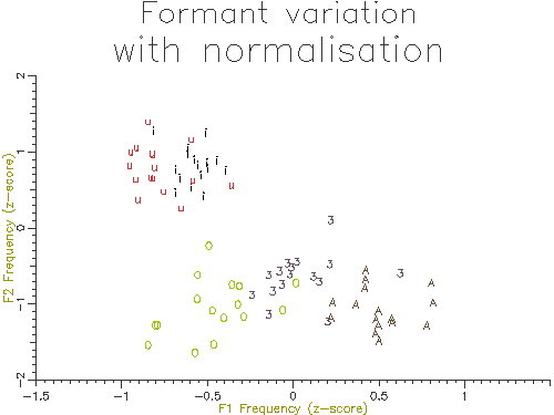
Figure 4.11 - Vowel analysis with normalisation
5. Data Analysis
We have collected together a range of tools for measuring formant frequencies from annotated speech signals. In this section we will look at how we might use those tools to establish the likelihood of various experimental hypotheses using techniques of inferential statistics.
Comparison of means (univariate)
As can be seen from the formant frequency distributions shown in Figures 4-3 to 4-8, typical formant distributions for a single segment show a fairly normal shape. Thus it is reasonable for us to use a parametric method for comparing the means of two samples. We'll show this kind of analysis through a worked example.
Is a vowel the same in two different contexts?
In this example we look at some instances of /i:/ vowels spoken in word final and word medial positions. We can use one of the scripts from section 4 (e.g. fmsummary4.sml) to extract this data from annotated recordings of a single speaker. Here we have divided it into two sets according to the context in which each vowel occurs:
| Word final |
|---|
"sse_f_02_02.sfs","iy/we", 418.8033, 1774.0710, 2394.6035 "sse_f_02_03.sfs","iy/security", 627.6675, 1651.4409, 2598.3047 "sse_f_02_04.sfs","iy/be", 463.7514, 1803.9850, 2568.7997 "sse_f_02_05.sfs","iy/be", 659.1691, 2073.7795, 2667.1369 "sse_f_02_14.sfs","iy/agency", 577.9793, 2376.8602, 2939.6063 "sse_f_02_16.sfs","iy/Gary", 538.9950, 2037.0008, 2349.4858 "sse_f_02_19.sfs","iy/tea", 572.1907, 2190.4421, 2744.6243 |
| Word medial |
"sse_f_02_05.sfs","iy/people", 533.8898, 2297.5439, 2762.3784 "sse_f_02_06.sfs","iy/alleviate", 412.0224, 2108.4677, 2812.5599 "sse_f_02_07.sfs","iy/evening", 351.8525, 2425.5254, 2915.9789 "sse_f_02_10.sfs","iy/diseases", 420.0742, 2093.2929, 2707.7623 "sse_f_02_15.sfs","iy/field", 489.4434, 2162.2629, 2611.0818 "sse_f_02_17.sfs","iy/unbeatable",455.4935, 2136.7220, 2748.7320 "sse_f_02_18.sfs","iy/leaves", 609.1624, 2063.6738, 2640.9705 |
A reasonable question to ask is whether there is a systematic difference in the formant frequencies of /i:/ across these two contexts (certainly F1 looks a bit higher and F2 looks a bit lower in word final position). For these data, the question we are asking is how likely it is that these two samples would have their means if they were really just two samples of the same underlying population of vowels. Thus the null hypothesis is that any observed difference in sample means is due to chance. If it turns out that the difference in means is rather unlikely due to chance alone then this suggests that there is a real effect of word position on the vowel.
To obtain the likelihood that a difference in sample means might have arisen by chance we can call on some mathematical analysis. Statisticians have simulated the drawing of samples of various sizes from a single population and have studied how how much natural variation we should expect in sample means from chance variation alone. Their knowledge about the likelihood of differences in sample means is summarised in the procedure called the t-test. We'll next demonstrate how to perform a t-test on our data.
We could perform a t-test using a statistics package, but here we will just use the Excel spreadsheet program (the OpenOffice Calc spreadsheet has the same functions). You may need to install the optional "Analysis ToolPak" (sic) to get the statistical functions.
Figure 5.1 shows the data in Excel, ready for the t-test values to be calculated:
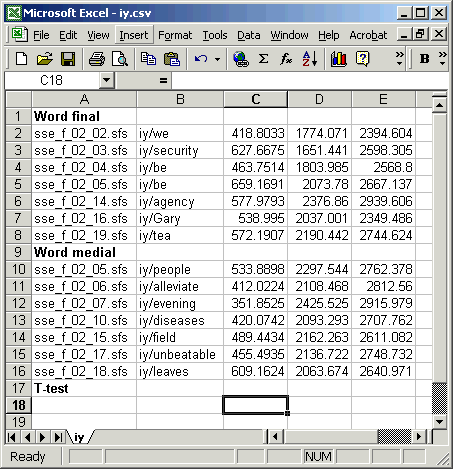
Figure 5.1 - Ready for t-test calculation in Excel
To enter the calculation for a t-test, use the TTEST(array1,array2,tails,type) function: array1 is the column of F1 values for word final, array2 is the column of F1 values for word medial, tails is 2 for test in which we don't care whether the frequencies should be higher or lower across conditions, type is 2 for when we believe that both sets have the same variance. Figure 5.2 shows the data in Excel, with the formula entered and copied under the F2 and F3 columns.
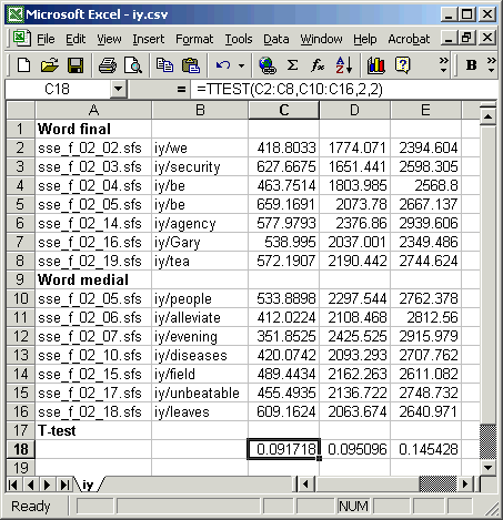
Figure 5.2 - T-test calculation in Excel
What is the interpretation of the t-test probabilities? The t-test shows us that for each formant there is about a 1 in 10 chance (p about 0.1) that the difference in the sample means could have arisen even if they were actually from the same underlying population. This is not good evidence that there is a real effect here: we'd expect this difference in observed means once in every ten experiments even if there were no effect to measure.
What level of probability would be small enough that we would believe there was a real effect? A very common level of significance is taken to be a probability less than 0.05; in other words we accept that there is an effect if the likelhood of the results occurring by chance is less than 1 in 20.
How do we combine the results of the three t-tests? This is a real problem. If we only looked at one variable then we would probably say we saw a real effect if the likelihood of the null hypothesis was less than 0.05. But because we are looking at more than one variable, it is more likely that we will get at least one variable showing a sigificant result (because we have conducted more experiments!). Thus we need to be more conservative in our choice of level of significance. The Bonferroni correction suggests that we should divide our level of significance by the number of tests, so if we are willing to accept a significant difference in either F1 or F2 we should look for p < 0.025, or if we are willing to accept a significant difference in F1, F2 or F3, we should look for a p < 0.017.
Using paired contexts
In the previous demonstration there was no obvious connection between the vowel contexts in each of the two sets, they were just two random samples of words in the recording. If we had planned the recording more carefully we could have constructed paired contexts, so that one of the pair would give us values in the first set, and one would give us a value in the second. For example we might have recorded words such as "happy/happiness", "silly/sillyness" where we could compare the vowel formant frequencies with and without an additional affix. This is called a "paired" test and is fundamentally more sensitive than the independent samples test we did above. In a paired test you are only looking for a systematic difference between members of each pair rather than a difference of means across the sets. In effect you are looking at the distribution of the hertz difference between the members of the pair, and the t-test establishes whether the mean of that difference across all pairs is significantly different from zero. The table below shows the idea.
| Word final | F1 value | Word medial | F1 | F1 Difference |
|---|---|---|---|---|
| happy | 278 | happiness | 358 | 80 |
| silly | 305 | silliness | 365 | 60 |
| ... | ... | ... | ... | ... |
In Excel we would enter the two columns of F1 values as the arguments to the TTEST() function, but choose a type parameter of 1 to calculate a paired test.
Comparison of means (multivariate)
Although the analysis presented in the last section is acceptable by most statisticians, it does have a remaining weakness. When we perform analysis on F1 and F2 separately we are assuming that there is no systematic correlation between the F1 and F2 values: that F1 and F2 are independent. Actually, for vowels this turns out not to be a bad assumption, with the correlation coefficient betwen F1 and F2 being quite low (about ρ=0.2). However, for completeness, we will look at ways to compare vowel distributions jointly in F1 and F2.
Plotting distributions on F1-F2 plane
First we'll look at graphing vowel samples on the F1-F2 plane, plotting a contour expressing one standard deviation in two-dimensions. The following script collects F1 and F2 frequencies from the five long monophthongs from a single speaker. It then plots these on a scatter graph and estimates the shape and size of an ellipse that characterises the distribution of values.
/* f1f2distributions.sml - collect and plot F1-F2 distributions */

/* raw data tables - one per vowel type */
var        t1f1[1:1000],t1f2[1:1000],t1cnt;
var        t2f1[1:1000],t2f2[1:1000],t2cnt;
var        t3f1[1:1000],t3f2[1:1000],t3cnt;
var        t4f1[1:1000],t4f2[1:1000],t4cnt;
var        t5f1[1:1000],t5f2[1:1000],t5cnt;

/* output file */
file    gop;

/* calculate trimmed mean */
function var trimmean(table,len)
{
    var table[];    /* array of values */
    var len;        /* # values */
    var    i,j,tmp;
    var    lo,hi;

    /* sort table */
    for (i=2;i<=len;i=i+1) {
        j = i;
        tmp = table[j];
        while (table[j-1] > tmp) {
            table[j] = table[j-1];
            j = j - 1;
            if (j==1) break;
        }
        table[j] = tmp;
    }

    /* find mean over middle portion */
    lo = trunc(0.5 + 1 + len/5);    /* lose bottom 20% */
    hi = trunc(0.5 + len - len/5);    /* lose top 20% */
    j=0;
    tmp=0;
    for (i=lo;i<=hi;i=i+1) {
        tmp = tmp + table[i];
        j = j + 1;
    }
    if (j > 0) return(tmp/j) else return(ERROR);
}

/* get trimmed mean formant value for a segment */
function var measure_trimmed_mean(stime,etime,pno)
{
    var    stime;    /* start time */
    var    etime;    /* end time */
    var    pno;    /* FM parameter # */
    var    t;        /* time */
    var af[1:1000];    /* array of values */
    var    nf;        /* # values */

    /* calculate trimmed mean */
    nf=0;
    t=next(FM,stime);
    while ((t < etime)&&(nf < 1000)) {
        nf = nf+1;
        af[nf] = fm(pno,t);
        t = next(FM,t);
    }

    return(trimmean(af,nf));
}

/* record details of a single segment */
function var recordsegment(stime,etime,tf1,tf2,tcnt)
var    tf1[];
var    tf2[];
var tcnt;
{
    var stime,etime;
    var vf1,vf2

    vf1 = measure_trimmed_mean(stime,etime,5);
    vf2 = measure_trimmed_mean(stime,etime,8);
    if (vf1 && vf2) {
        tcnt=tcnt+1;
        tf1[tcnt] = vf1;
        tf2[tcnt] = vf2;
    }
}

/* plot ellipse for 2D gaussian */
function var plotellipse(sx,sy,sxy)
{
    stat sx,sy,sxy;
    var    xdata[0:360];
    var    ydata[0:360];
    var    a,cnt;
    var    rho;        /* correlation coeff */
    var    lam1,lam2;    /* eigenvalues */
    var    ax1,ax2;    /* axis lengths */
    var    alpha;        /* ellipse angle */

    /* get parameters of ellipse from distribution */
    rho = (sxy.mean-sx.mean*sy.mean)/(sx.stddev * sy.stddev);
    lam1 = 0.5 * (sx.variance+sy.variance+ \
        sqrt((sx.variance-sy.variance)*(sx.variance-sy.variance)+ \
        4*sx.variance*sy.variance*rho*rho));
    lam2 = 0.5 * (sx.variance+sy.variance- \
        sqrt((sx.variance-sy.variance)*(sx.variance-sy.variance)+ \
        4*sx.variance*sy.variance*rho*rho));
    ax1 = 2*sqrt(0.35*lam1);    /* about 70% inside */
    ax2 = 2*sqrt(0.35*lam2);
    alpha = 0.5*atan2(2*rho*sx.stddev*sy.stddev,sx.variance-sy.variance);

    /* calculate locus of ellipse */
    cnt=0;
    for (a=0;a<=6.3;a=a+0.05) {
        xdata[cnt] = sx.mean + ax1*cos(a)*cos(alpha) - ax2*sin(a)*sin(alpha);
        ydata[cnt] = sy.mean + ax1*cos(a)*sin(alpha) + ax2*sin(a)*cos(alpha);
        cnt=cnt+1;
    }

    /* plot ellipse */
    plotparam("type=line");
    plotparam("char=");
    plotxdata(xdata,0);
    plot(gop,1,ydata,cnt);
}

/* plot F1-F2 for segment */
function var plotf1f2segment(label,tf1,tf2,tcnt)
var tf1[];
var tf2[];
{
    var        tcnt;
    string    label;
    stat    sx,sy,sxy;
    var        i;

    plotparam("type=point");
    plotparam("char="++label);

    /* plot raw samples */
    plotxdata(tf1,0);
    plot(gop,1,tf2,tcnt);

    /* collect statistics on samples */
    for (i=1;i<=tcnt;i=i+1) {
        sx += tf1[i];
        sy += tf2[i];
        sxy += tf1[i]*tf2[i];
    }

    /* plot ellipse at 1 standard deviation */
    plotellipse(sx,sy,sxy);
}

/* plot F1-F2 graph */
function var plotf1f2()
{
    openout(gop,"|dig");
    plottitle(gop,"Vowel variability");
    plotparam("title=single speaker, all contexts");
    plotparam("xtitle=F1 Frequency (Hz)");
    plotparam("ytitle=F2 Frequency (Hz)");
    plotparam("type=point");
    plotaxes(gop,1,200,800,500,2500);

    /* for each segment in turn */
    plotf1f2segment("i",t1f1,t1f2,t1cnt);
    plotf1f2segment("u",t2f1,t2f2,t2cnt);
    plotf1f2segment("3",t3f1,t3f2,t3cnt);
    plotf1f2segment("A",t4f1,t4f2,t4cnt);
    plotf1f2segment("O",t5f1,t5f2,t5cnt);

    close(gop);
}

/* for each file to be processed */
main {
    var    num;    /* # annotated regions */
    var    i;
    var stime,etime;
    var    scode;
    string    label;

    /* report file */
    num = numberof(".");
    print#stderr "File ",$filename," has ",num," annotations\n";

    /* for each annotation */
    for (i=1;i<=num;i=i+1) {
        stime = timen(".",i);
        etime = stime + lengthn(".",i);
        label = matchn(".",i);
        switch (label) {
        case "i:": recordsegment(stime,etime,t1f1,t1f2,t1cnt);
        case "u:": recordsegment(stime,etime,t2f1,t2f2,t2cnt);
        case "3:": recordsegment(stime,etime,t3f1,t3f2,t3cnt);
        case "A:": recordsegment(stime,etime,t4f1,t4f2,t4cnt);
        case "O:": recordsegment(stime,etime,t5f1,t5f2,t5cnt);
        }
    }
}

/* summarise collected data */
summary {
    /* plot graph */
    plotf1f2();
}
|
Figure 5.3 shows the output of the script. The data used is rather noisy because it has been collected over a large number of different contexts. The ellipses contain about 70% of the data values, analogous to one standard deviation containing 70% of a normal distribution.
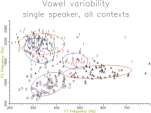
Figure 5.3 - Vowel distribution on F1-F2 plane
Comparing the centroids of two vowel samples on the F1-F2 plane
Looking carefully at Figure 5.3 you will see that there is a large overlap in the distributions of /i:/ and /u:/ on the F1-F2 plane. We will now consider how we might perform a statistical test that determines whether these two samples are really distinct or come from the same underlying population (we are pretty sure that /i:/ and /u:/ are different, of course!). Rather than use two t-tests on the F1 values and the F2 values separately, we will show how to perform a single test that uses F1 and F2 jointly.
A statistical test on one random variable is called a "univariate" test; while a statistical test on 2 or more variables is called "multivariate". In this case we need to use the multivariate equivalent of the t-test, and this is called "Hotelling's T2 test".
The script below collects information about the F1 and F2 distribution of two vowels and calculates the value of Hotelling's T2 statistic on the two samples.
/* f1f2compare.sml - calculate Hotelling's T-squared on vowel pair */

/* vowels to measure */
string    label1;
string    label2;

/* raw data tables - one per vowel type */
var        t1f1[1:1000],t1f2[1:1000],t1cnt;
var        t2f1[1:1000],t2f2[1:1000],t2cnt;

/* calculate trimmed mean */
function var trimmean(table,len)
{
    var table[];    /* array of values */
    var len;        /* # values */
    var    i,j,tmp;
    var    lo,hi;

    /* sort table */
    for (i=2;i<=len;i=i+1) {
        j = i;
        tmp = table[j];
        while (table[j-1] > tmp) {
            table[j] = table[j-1];
            j = j - 1;
            if (j==1) break;
        }
        table[j] = tmp;
    }

    /* find mean over middle portion */
    lo = trunc(0.5 + 1 + len/5);    /* lose bottom 20% */
    hi = trunc(0.5 + len - len/5);    /* lose top 20% */
    j=0;
    tmp=0;
    for (i=lo;i<=hi;i=i+1) {
        tmp = tmp + table[i];
        j = j + 1;
    }
    if (j > 0) return(tmp/j) else return(ERROR);
}

/* get trimmed mean formant value for a segment */
function var measure_trimmed_mean(stime,etime,pno)
{
    var    stime;    /* start time */
    var    etime;    /* end time */
    var    pno;    /* FM parameter # */
    var    t;        /* time */
    var af[1:1000];    /* array of values */
    var    nf;        /* # values */

    /* calculate trimmed mean */
    nf=0;
    t=next(FM,stime);
    while ((t < etime)&&(nf < 1000)) {
        nf = nf+1;
        af[nf] = fm(pno,t);
        t = next(FM,t);
    }

    return(trimmean(af,nf));
}

/* record details of a single segment */
function var recordsegment(stime,etime,tf1,tf2,tcnt)
var    tf1[];
var    tf2[];
var tcnt;
{
    var stime,etime;
    var vf1,vf2

    vf1 = measure_trimmed_mean(stime,etime,5);
    vf2 = measure_trimmed_mean(stime,etime,8);
    if (vf1 && vf2) {
        tcnt=tcnt+1;
        tf1[tcnt] = vf1;
        tf2[tcnt] = vf2;
    }
}

/* calculate mean and covariance */
function var covar(a1,a2,cnt,amean,acov)
var amean[],acov[];
{
    var        a1[],a2[],cnt;
    var     i;
    stat    s1,s2;

    for (i=1;i<=cnt;i=i+1) {
        s1 += a1[i];
        s2 += a2[i];
    }
    amean[1]=s1.mean;
    amean[2]=s2.mean;
    for (i=1;i<=cnt;i=i+1) {
        a1[i] = a1[i] - s1.mean;
        a2[i] = a2[i] - s2.mean;
    }
    clear(acov);
    for (i=1;i<=cnt;i=i+1) {
        acov[1] = acov[1] + a1[i]*a1[i];
        acov[2] = acov[2] + a1[i]*a2[i];
        acov[3] = acov[3] + a2[i]*a1[i];
        acov[4] = acov[4] + a2[i]*a2[i];
    }
    for (i=1;i<=4;i=i+1) acov[i] = acov[i] / (cnt-1);
}

/* calculate Hotelling's T-squared */
function var hotelling(v11,v12,v1cnt,v21,v22,v2cnt)
var    v11[],v12[],v1cnt;
var    v21[],v22[],v2cnt;
{
    var    i;
    var mean1[1:2];
    var    cov1[1:4];
    var mean2[1:2];
    var cov2[1:4];
    var    dmean[1:2];
    var    cov[1:4];
    var    icov[1:4];
    var    t2;

    /* get individual means and covariances */
    covar(v11,v12,v1cnt,mean1,cov1);
    covar(v21,v22,v2cnt,mean2,cov2);

    /* get difference in means */
    dmean[1] = mean2[1]-mean1[1];
    dmean[2] = mean2[2]-mean1[2];

    /* combine covariances */
    for (i=1;i<=4;i=i+1) {
        cov[i] = ((v1cnt-1)*cov1[i] + (v2cnt-1)*cov2[i])/(v1cnt+v2cnt-2);
    }

    /* invert covariance */
    icov[1]=cov[4]/(cov[4]*cov[1]-cov[2]*cov[3]);
    icov[2]=(1-cov[1]*icov[1])/cov[2];
    icov[3]=(1-cov[1]*icov[1])/cov[3];
    icov[4]=cov[1]*icov[1]/cov[4];

    /* put t2 together in parts */
    t2 = 0;
    t2 = t2 + dmean[1]*(dmean[1]*icov[1]+dmean[2]*icov[3]);
    t2 = t2 + dmean[2]*(dmean[1]*icov[2]+dmean[2]*icov[4]);
    t2 = (v1cnt*v2cnt*t2)/(v1cnt+v2cnt);

    return(t2);
}

/* get names of vowels to measure */
init {
    print "Enter vowel label 1 : ";
    input label1;
    print "Enter vowel label 2 : ";
    input label2;
}

/* for each file to be processed */
main {
    var    num;    /* # annotated regions */
    var    i;
    var stime,etime;
    var    scode;
    string    label;

    /* report file */
    num = numberof(".");
    print#stderr "File ",$filename," has ",num," annotations\n";

    /* for each annotation */
    for (i=1;i<=num;i=i+1) {
        stime = timen(".",i);
        etime = stime + lengthn(".",i);
        label = matchn(".",i);
        if (compare(label,label1)==0) {
            recordsegment(stime,etime,t1f1,t1f2,t1cnt);
        }
        else if (compare(label,label2)==0) {
            recordsegment(stime,etime,t2f1,t2f2,t2cnt);
        }
    }
}

/* summarise collected data */
summary {
    var t,f;

    print "Analysis summary:\n"
    print "  Number of files = ",$filecount:1,"\n";
    print "  Number of instances of /",label1,"/ = ",t1cnt:1,"\n";
    print "  Number of instances of /",label2,"/ = ",t2cnt:1,"\n";

    /* calculate Hotelling T-squared statistic */
    t = hotelling(t1f1,t1f2,t1cnt,t2f1,t2f2,t2cnt);
    print "  Hotelling T-squared statistic =",t:5:2,"\n";

    /* report equivalent F statistic */
    f=(t1cnt+t2cnt-3)*t/((t1cnt+t2cnt-2)*2);
    print "  For significance find probability that F(2,", \
            (t1cnt+t2cnt-3):1,") >",f:5:2,"\n";
}
|
When this script is run on the data used to produce Figure 5.3 on the vowels /i:/ and /u:/, the result is:
Analysis summary:
  Number of files = 30
  Number of instances of /i:/ = 192
  Number of instances of /u:/ = 39
  Hotelling T-squared statistic = 18.80
  For significance find probability that F(2,228) > 9.36
From this output you can see that the Hotelling's T2 statistic is 18.8 for these two vowels. To interpret this number we need to know how often this value would occur for samples of the size we used if there were no underlying difference between these vowels. To turn the T2 statistic into a probability we can use the fact that its distribution follows the same shape as the F distribution of a particular configuration (basically for a p-variate sample of df= n, the F statistic is (n-p)/p(n-1) times the T2 statistic). So in this case, the likelihood of a T2 of 18.8 is equivalent to the likelihood of an F(2,228) statistic of 9.36. Since in general we are only interested in the significance of the statistic, here are a few critical values from the F-distribution F(2,n):
| F statistic | p < 0.05 | p < 0.01 |
|---|---|---|
| F(2,10) | 4.1 | 7.56 |
| F(2,20) | 3.49 | 5.85 |
| F(2,50) | 3.19 | 5.08 |
| F(2,100) | 3.10 | 4.85 |
| F(2,200) | 3.06 | 4.77 |
| F(2,500) | 3.04 | 4.71 |
Since the likelihood of F(2,200) being greater than 4.77 is less than 0.01, we can be sure that the likelihood of F(2,228) being greater than 9.36 is much less than 0.01. Thus there is a significant difference between these two distributions (phew!).
The procedure above could be extended to work with F1, F2 and F3 if required. But if you wanted to test if 3 or more samples came from the same population (rather than just 2 in this case) you'd need to perform a multivariate analysis of variance or MANOVA.
Bibliography
The following have been used in the development of this tutorial:
- Maria Isabel Ribeiro, Gaussian Probability Density Functions: Properties and Error Characterization at http://omni.isr.ist.utl.pt/~mir/pub/probability.pdf
- Hotelling's T2 test at http://www.itl.nist.gov/div898/handbook/pmc/section5/pmc543.htm
- Critical F Distribution Calculator at http://www.psychstat.smsu.edu/introbook/fdist.htm
Feedback
Please report errors in this tutorial to sfs@pals.ucl.ac.uk. Questions about the use of SFS can be posted to the SFS speech-tools mailing list.