
SFS/WASP Help File
| Program: | Vs 1.60 |
| Help file: | Vs 1.7 |
Contents:
Internet links:
WASP is a program for the recording, display and analysis of speech. With WASP you can record and replay speech signals, save them and reload them from disk, edit annotations, display spectrograms and a fundamental frequency track, and print the results.
WASP is a simple application that is complete in itself but which is also designed to be compatible with the Speech Filing System (SFS) tools for speech research.
Controls
Toolbar
- Open file. Use to open an existing signal file stored on disk. Supports standard Microsoft RIFF format (.WAV files) as well as SFS file format.
- Save file. Use to save a new recording to a disk file, or to save an existing signal file under a new name. WASP can save in RIFF or SFS format. Note that only the signal can be stored in RIFF files, so that any annotations will be lost.
- Print. Use to reproduce the current display on the printer. Note that printouts are produced in landscape format by default. Cursors are not printed.
- Record. Use to record a new speech signal. Selection of the input device and input sensitivity must be made through the use of the system volume controls, see recording below.
- Play (or [space] key). Use to replay the region of the current signal displayed or between cursors. Selection of the output device and volume must be made through the use of the system volume controls.
- Stop. Stops replay.
- Waveform. Use to display an amplitude waveform graph of the speech signal.
- Wideband Spectrogram. Use to display a wide bandwidth spectrogram of the speech signal. This is calculated dynamically from the speech signal as required.
- Narrowband Spectrogram. Use to display a narrow bandwidth spectrogram of the speech signal. This is calculated dynamically from the speech signal as required.
- Fundamental frequency. Use to display a fundamental frequency track ("pitch track") for the speech signal. This is calculated once when first requested.
- Pitch marks. Use to display glottal closure markers ("pitch marks") for the speech signal. This is calculated once when first requested.
- Annotations. Use to display any annotations associated with the speech signal. Annotations can be added using the cursors and saved to SFS files.
- Scroll left (Left arrow or 'L' key). Use to move the display to an earlier part of the signal.
- Zoom in (Down arrow or 'Z' key). Use to focus the display on a smaller section of the displayed signal. To zoom in, first set the area of interest with left and right cursors.
- Zoom out (Up arrow or 'U' key). Use to undo one level of zoom.
- Scroll right (Right arrow or 'R' key). Use to move the display to a later part of the signal.
Other menu options
- File properties. Use to set some information fields in the header of the SFS file. This information is saved with the speech data in the file. The Speaker and Token fields also appear on printouts. Not applicable to Audio (WAV) files.
- View properties. Use to control some of the display formatting. Options allow the SFS history fields and the SFS numbers for the data items to be displayed. Unless you are familiar with SFS, these are probably not of much interest and can be turned off. The grid option overlays a grid on the spectrogram and fundamental frequency display to make measurements easier. However they do tend to obscure the displays. You can also set the maximum displayed frequency for spectrograms.
- View statistics. Report various statistics of the signal. See section below for details.
- Crop Signal. Use to discard region of signal outside cursors or outside current display. You can use this option to select one part of a longer recording before saving it to a new file. If you need to select multiple parts of a recording, first save it to file, then reload it after each crop and save. There is no other way back to the original recording after you have selected crop.
- Save Section to File. Use to save the region identified between the cursors to a new file. WASP can only save to audio (WAV) files.
- Edit/Copy Display. Copies the current display to the clipboard so that you can paste the image into other programs. Note that the image size and shape is defined by the current size and shape of the window. Also the colour depth is set by the properties of the current display.
Other replay commands
- 'I' key. Replay from beginining of file to start of displayed section.
- 'O' key. Replay section of signal before left cursor or before start of displayed section.
- 'P' key. Replay section of signal between left and right cursors or displayed section.
- '[' key. Replay section of signal after right cursor or after end of displayed section.
- ']' key. Replay from end of displayed section to end of file.
- Signal/Play File. Replay entire file.
Cursors and Annotations
With a waveform loaded and displayed, you can set left and right cursors using the left and right mouse buttons. The left cursor is blue, the right cursor is green. These cursors indicate the start and stop time for various operations:
- for replay the signal replayed is the region between the cursors.
- for zoom in the region between the cursors is expanded to fill the display.
- for scroll left the right cursor becomes the new right edge of the display.
- for scroll right the left cursor becomes the new left edge of the display.
- for annotation the entered labels are placed at times specified by the left or right cursors.
To enter an annotation, first press the letter 'A' (for annotation at the left cursor) or 'B' (for annotation at the right cursor) then type in the label and press the RETURN key when done. You will see the characters you type appear in the status bar. You can edit a label being entered with the BACKSPACE key. You can cancel an annotation entry by pressing ESCAPE. You can change an annotation by entering a new annotation at the same place. You can delete an annotation by entering an empty annotation at the same place.
The time at which the left and right cursors are located is displayed in the status bar. For convenience, the interval between the cursors is also displayed, as well as the reciprocal of that interval. These may be of use to estimate durations and frequencies from the signal.
You can remove a cursor by clicking the mouse button twice at the same location.
Information about the location of the cursors is displayed at the right of the status bar. The times of the left and right cursor are displayed, also the interval between them expressed in seconds and Hertz, and finally the value of the fundamental frequency track under the left cursor.
Signal statistics
The View|Statistics menu option displays various statistics of the signal for the whole file and for the selected region:
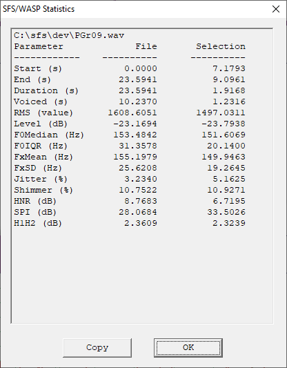
Some statistics require that a pitch track or pitch marks are calculated first.
Statistics are as follows:
- Start
- Time in signal where analysis starts.
- End
- Time in signal where analysis ends.
- Duration
- Duration of signal analysed.
- Voiced
- Duration of signal where signal is voiced (from pitch marks).
- RMS
- Root-mean-square sample amplitude.
- Level
- RMS level expressed in deciBels. Reference is maximum amplitude sinusoid.
- F0Median
- Median fundamental frequency (from pitch track)
- F0IQR
- Inter-quartile range of fundamental frequency (from pitch track)
- FxMean
- Mean fundamental frequency (from pitch marks)
- FxSD
- Standard deviation of fundamental frequency (from pitch marks).
- Jitter
- Perturbation of glottal cycle durations, calculated per pitch period in window of 5 periods (from pitch marks).
- Shimmer
- Perturbation of glottal cycle amplitudes, calculated per pitch period in window of 5 periods (from pitch marks).
- HNR
- Harmonic-to-noie ratio, calculated per pitch period in window of 5 periods (from pitch marks).
- SPI
- Soft phonation index, ratio of high frequency (1600-4500Hz) to low-frequency (70-1600Hz) energy, calculated over pitch periods (from pitch marks).
- H1H2
- Ratio of amplitude of first two harmonics, calculated per pitch period in window of 5 periods (from pitch marks).
Recording
Most PCs have two input lines, one designed for a microphone input and one designed for a 'line' level input (from e.g. a tape recorder). Some PCs are also able to record output from audio CDs played in the computer. Once your signal source is connected to the computer, you need to select it using the Volume Control application. This can be found under the Start/Programs/Accessories/Multimedia menu on Windows 95/98/NT systems.
To record from a microphone:
- ensure that it is connected to the microphone input to the PC.
- ensure that the microphone input device is selected in volume control.
- ensure that the input volume and overall record volume are at moderate levels.
- request the record menu option in WASP and select 'Test Levels' to check that signals are getting to the program.
- adjust the volume controls so that at no time does the peak level reach the right hand side of the display when recording.
- select 'Record' to record the signal, 'Stop' once complete, and then 'OK'. The waveform should be displayed in the main window.
In the WASP record dialogue, you can adjust the recording quality by changing the sampling rate. The default rate of 16000 samples per second with 16-bit resolution has been chosen to be most useful for the production of speech spectrograms. Not all PCs support acquisition at 16000 samples per second. You may find it necessary to record at 22050 samples/second or at 11025 samples/second.
Displays
Waveform
A waveform is a graph of signal amplitude (on the vertical axis) against time (on the horizontal axis). Conventionally, the zero line is taken to mean no input: in terms of a microphone this would imply that the sound pressure at the microphone was the same as atmospheric pressure. Positive and negative excursions can then be considered pressure fluctuations above and below atmospheric pressure. For speech signals these pressure fluctuations are very small, typically less than +/- 1/1000000 of atmospheric pressure. The amplitude scale used on waveform displays merely records the size of the quantised amplitude values captured by the Analogue-to-Digital converter in the PC. These have a maximum range of -32,768 to +32,767. If you observe values close to these on the display, it is likely that the input signal is overloaded.
Wideband spectrogram
A spectrogram is a display of the frequency content of a signal drawn so that the energy content in each frequency region and time is displayed on a grey scale. The horizontal axis of the spectrogram is time, and the picture shows how the signal develops and changes over time. The vertical axis of the spectrogram is frequency and it provides an analysis of the signal into different frequency regions. You can think of each of these regions as comprising a particular kind of building block of the signal. If a building block is present in the signal at a particular time then a dark region will be shown at the frequency of the building block and the time of the event. Thus a spectrogram shows which and how much of each building block is present at each time in the signal. The building blocks are, in fact, nothing more than sinusoidal waveforms (pure tones) occuring with particular repetition frequencies. Thus the spectrogram of a pure tone at 1000Hz will consist of a horizontal black line at 1000Hz on the frequency axis. Such a signal only contains a single type of building block: a sinusoidal signal at 1000Hz.
Wideband spectrograms use coarse-grained regions on the frequency axis. This has two useful effects: firstly it means that the temporal aspects of the signal can be made clear - we can see the individual larynx closures as vertical striations on a wide band spectrogram; secondly it means that the effect of the vocal tract resonances (called formants) can be seen clearly as black bars between the striations - the resonances carry on vibrating even after the larynx pulse has passed though the vocal tract. The bandwidth for the wideband display is fixed at 300Hz.
Narrowband spectrogram
Narrowband spectrograms use fine-grained regions on the frequency axis. This has two main effects: firstly fine temporal detail is lost which means that the individual larynx pulses are no longer seen; secondly fine frequency structure is brought out consisting of the harmonics of the larynx vibration as filtered by the resonances of the vocal tract. This kind of display is most useful for the study of slowly varying properties of the signal, such as fundamental frequency. The bandwidth for the narrowband display is fixed at 45Hz.
Fundamental frequency track
The fundamental frequency track shows how the pitch of the signal varies with time. Pitch is properly a subjective attribute of the signal, but it is closely related to the repetition frequency of a periodic waveform. Thus if a signal has a waveform shape that repeats in time (such as a simple vowel) then we perceive a pitch related to how long the signal takes to repeat. A signal with a long repetition period (low repetition frequency) has a low pitch, while a signal with a short repetion period (high repetition frequency) has a high pitch. The proper name for the repetition frequency of periodic waveforms is called the fundamental frequency because this frequency has an important role in determining which frequency components are present in a periodic signal. A signal that is periodic at F Hz, can only have frequency components at F, 2F, 3F, ...; these are called the harmonic components (or just harmonics) of the signal.
The pitch estimation algorithm used in WASP is called RAPT ("A robust algorithm for pitch tracking", David Talkin).
Note that all algorithms for estimating the fundamental frequency from the speech signal do fail on some occasions. This is because of the complexity of the speech signal and the influence of any interfering noise. Where the algorithm is unable to determine any effective periodicity in the signal, no fundamental frequency estimate is displayed. The algorithm is optimised for human speech signals, so may fail to find the correct pitch for musical instruments and other sounds.
Pitch marks
The pitch marks display shows estimated times of glottal closures (Tx). These indicate times at which the vocal folds close in each voicing cycle. The pitch mark algorithm used in WASP is called REAPER, also by David Talkin.
Annotations
Annotations are simply text labels that are associated with a particular time in the speech signal. They may be used to mark the boundaries between words or phonetic segments or to indicate the presence of specific events. Annotations are automatically saved and restored with the speech signal when you choose to use SFS format files. To perform additional processing with these labels you need to use some of the SFS tools such as anlist, andict, or sml. See the SFS Web Pages for more information.
Want to learn more?
If you find the study of speech interesting and would like to know more, why not visit the Internet Institute of Speech and Hearing at www.speechandhearing.net ? There you will find tutorials, reference material, laboratory experiments and contact details of professional organisations.
Bug reports
Please send suggestions for improvements and reports of program faults to SFS@phon.ucl.ac.uk.
Please note that we are unable to provide help with the use of this program.
Copyright
WASP is not public domain software, its intellectual property is owned by Mark Huckvale, University College London. However WASP may be used and copied without charge as long as the program and help file remain unmodified and continue to carry this copyright notice. Please contact the author for other licensing arrangements. WASP carries no warranty of any kind, you use it at your own risk.
Wasp contains fundamental frequency estimation code developed by David Talkin and Derek Lin as part of the Entropic Signal Processing System and is used under licence from Microsoft.
Wasp artwork originally from www.webdog.com.au with thanks.