10. Tips and Tricks
Topics
- Uniquely Identifying Subjects
It can sometimes prove useful to assign a unique identifier to each of your subjects. For example you may want to store multiple results per subject in the database and then match them up later. One way to do this is to generate a unique code for the subject when they first access your page then use the same code to identify the all measurements for that subject in the uploaded data.
The Javascript library uuid.js contains functions to generate a unique user identifier code based on the date and time at which the subject accessed your page. The library can be found in the "include" folder on the course web site. To generate a UUID, use code such as:
<script src="uuid.js"></script>
...
<script>
var uuid=generateUuid();
</script>
You can see a generated UUID by clicking the button below:
- Data Preparation
Before performing any inferential statistics on your measurements you should check your data is well distributed. Taking means or standard deviations or running t-tests on data which is highly skewed or has many outliers will not give you sensible results.
Conditioning
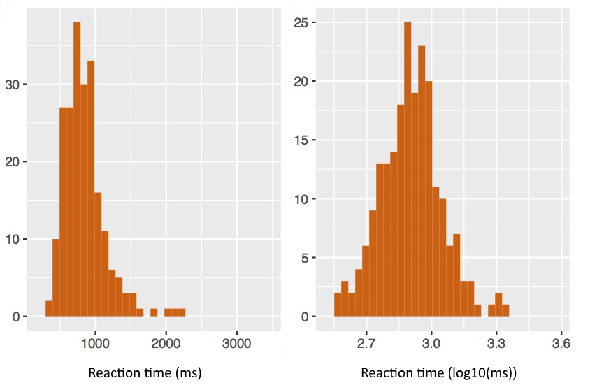
The goal of data conditioning is to ensure your data samples follow a distribution which is close to normal. A starting point is often to plot a histogram to check the shape and symmetry of the distribution.
Reaction times are commonly poorly distributed since there is a strong lower limit of zero, but no upper limit. Reaction time distributions often have a long tail of longer-time measurements. A common conditioning step is to apply a log transform.
Similarly, percentage scores often have odd distributions, since they have a fixed floor of 0% and a fixed ceiling of 100%. It is usually not appropriate to perform t-tests or ANOVAs on percentages. A common conditioning step is to convert them to log-odds. The log odds of some proportion p is just log(p/(1-p)), where 0 < p < 1. This maps p into a range from −∞ to +∞ and is commonly more normally distributed.
Outliers are another common problem. For reaction times it is a good idea to have an upper limit of an acceptable reaction time - say a second or two, so that you can reject very long and unlikely reaction times right from the beginning. One simple rule you can use to remove outliers is to calculate the inter-quartile range of the data, then reject any value which is more than 1.5*IQR below the 25th percentile or above the 75th percentile.
<script src="include/simple-statistics.js"></script>
...
// outlier removal
function outlier_filter(data) {
   var q25=ss.quantile(data,0.25);
   var q75=ss.quantile(data,0.75);
   var iqr=q75-q25;
   var lo=q25-1.5*iqr,hi=q75+1.5*iqr;
   var odata=[];
   for (var i=0;i<data.length;i++) {
      if ((lo <= data[i]) && (data[i] <= hi))
         odata.push(data[i]);
   }
   return(odata);
}
Repeated Measures
A common pitfall in inferential statistics is pseudo-replication, that is treating repeated responses to the same stimulus by the same subject as independent data points. If your experiment collects more than one response for each condition then you have repeated measures. Although statistical methods exist which cope with the non-independence of repetitions, perhaps the best advice is to average across repetitions before submitting your data for analysis. That is for each subject you will record only one number for each condition, then submit the now independent values across subjects to null-hypothesis testing.
The following example code shows how you might average the responses within subjects for each condition. You might use this to find an average reaction time, say, for each condition for each subject.
<script src="include/simple-statistics.js"></script>
...
// callback function for UCLLoad
// assume "subj" field contains unique UUID
// assume "cond" field has condition identifier
// assume "resp" field has a score or time to average
function process(data) {
   var txt="";
   if (data==null) {
      txt = "Request failed";
   }
   else {
      var sdata=aggregate(data);
      for (var i=0;i<sdata.length;i++) {
         txt += "subj="+sdata[i].subj;
         txt += " cond="+sdata[i].cond;
         txt += " resp="+sdata[i].resp+"\n";
      }
   }
   document.getElementById("summary").innerHTML=txt;
}
// aggregate entries for the same subject by
// computing mean response for each condition
function aggregate(data) {
   var sdata=[];
   // convert resp into array for subject & condition
   for (var i=0;i<data.length;i++) {
      var j;
      for (j=0;j<sdata.length;j++) {
         if ((sdata[j].subj==data[i].subj)
              &&(sdata[j].cond==data[i].cond)) break;
      }
      if (j<sdata.length)
         sdata[j].resp.push(data[i].resp);
      else
         sdata.push({ subj:data[i].subj,
            cond:data[i].cond, resp:[ data[i].resp ] });
   }
   // average out values
   for (var j=0;<sdata.length;j++) {
      sdata[j].resp = ss.mean(sdata[j].resp);
   }
   return(sdata);
}
Within Subject Designs
Many web experiments are actually performed as within-subject designs, that is each subject sees all conditions and so inference can be made from the difference in scores across conditions rather than the absolute value of the scores for each condition. Within-subject designs are more powerful because you are taking out of the analysis the absolute average performance of each subject across conditions.
Say, for example that you test your subjects on two conditions. You could collect all the scores for condition 1 and all the scores for condition 2 and perform an independent samples t-test. However a better strategy would be to collect the differences between condition 1 and condition 2 for each subject in turn, then use a one-sample t-test to investigate whether the mean difference between conditions is significantly different to zero.
- Doing Statistics
The following sections show how some simple inferential statistics may be performed in JavaScript. This allows you to include "live" statistical analysis in your experimental report - that is an analysis that changes as more people perform your experiment. These sections make use of the "Simple Statistics" library we met in week 8, and a course-specific library of JavaScript functions for computing the likelihood of some common statistics such as t-scores, F-ratios and chi-square scores. This library is called probability.js and may be found in the include folder on the web site.
Linear Regression and Correlation
Linear regression and correlation look at the relationship between two continuous variables: x and y. Linear regression finds the best values for a formula that predicts y from x using a linear function, that is the parameters m and b in the formula y = mx + b. Correlation provides a measure of the quality of that regression line. The correlation coefficient r ranges from -1 for a perfect negative correlation, 0 for no correlation to +1 for a perfect positive correlation. The value r2 is a measure of the degree of variability in y that is "explained" by x. High values of r2 mean that x and y are strongly related, but do not mean that x causes y.
Linear regression can be performed by the Simple Statistics function ss.linearRegression(data) the correlation coefficient can be calculated using the function ss.sampleCorrelation(x,y). A test for the significance of a correlation coefficient can be made by computing a t statistic then finding its likelihood in a cumulative t distribution with the appropriate degrees of freedom. An example is given below:
<script src="include/simple-statistics.js"></script>
<script src="include/probability.js"></script>
...
// perform linear regression, estimate correlation coefficient
function regression(x,y) {
    var table=[];
    for (var i=0;i<x.length;i++) table.push([ x[i],y[i] ]);
    var reg=ss.linearRegression(table);
    var rho=ss.sampleCorrelation(x,y);
    var df=x.length-2;
    var tval=rho*Math.sqrt(df/(1-rho*rho));
    var p=2*probability.tcdf(-Math.abs(tval),df);
    return({ m:reg.m, b:reg.b, rho:rho, df:df, tval:tval, p:p });
}
var x=[43,21,25,42,57,59];
var y=[99,65,79,75,87,81];
var res=regression(x,y);
console.log("Regression returns: "+JSON.stringify(res));
Which prints:Regression returns: {"m":0.385,"b":65.141,"rho":0.529,"df":4,"tval":1.249,"p":0.2798}t-tests
t-tests may be performed by the functions ss.tTest() and ss.tTestTwoSample() found in the simple statistics library. However these functions only return the t-statistic. To estimate a p-value from the t-statistic you need to look up the t-value in the cumulative t-distribution for the given numbers of degree of freedom in your samples using the probability library. For a given t-value tval and degrees of freedom df, the (one-tailed) p-value is just probability.tcdf(-Math.abs(tval),df), while the two-tailed p-value is twice as large.
You can try out the probability calculator using the converter below:
t-Statistic probability calculator t-Statistic Degrees of freedom For example, say you had a within samples design and for each subject you recorded two mean scores: one for condition 1 and one for condition 2. You might want to calculate the t score for the difference in means in paired samples and then estimate a p-value like this:
<script src="include/simple-statistics.js"></script>
<script src="include/probability.js"></script>
...
// callback function for UCLLoad
// assume "resp" field contains:
//    mean1=mean for condition1 and
//    mean2=mean for condition2
function process(data) {
   var txt="";
   if (data==null) {
      txt = "Request failed";
   }
   else {
      var diff=[];
      for (var i=0;i<data.length;i++) {
         diff.push(data[i].resp.mean1-data[i].resp.mean2);
      }
      var tval=ss.tTest(diff,0);
      var p=probability.tcdf(-Math.abs(tval),diff.length-1);
      txt = "Difference in means = " + ss.mean(diff);
      txt +=" t=" + tval + " p=" + p;
   }
   document.getElementById("performance").innerHTML=txt;
}
Here is a second example in which you have stored separate entries on the server for the two conditions and want to run an independent sample t-test. here we assume that the "cond" field contains the condition number and the "resp" field contains the actual performance score.
<script src="include/simple-statistics.js"></script>
<script src="include/probability.js"></script>
...
// callback function for UCLLoad
// assume "cond" field contains 1 or 2,
//   and "resp" field contains score
function process(data) {
   var txt="";
   if (data==null) {
      txt = "Request failed";
   }
   else {
      var samp1=[],samp2=[];
      for (var i=0;i<data.length;i++) {
         if (data[i].cond==1) samp1.push(data[i].resp);
         if (data[i].cond==2) samp2.push(data[i].resp);
      }
      var tval=ss.tTestTwoSample(samp1,samp2);
      var p=probability.tcdf(-Math.abs(tval),
                        samp1.length+samp2.length-2);
      txt = "Difference in means = " +
                        (ss.mean(samp1)-ss.mean(samp2));
      txt += " t=" + tval + " p=" + p;
   }
   document.getElementById("performance").innerHTML=txt;
}
One-way Analysis of Variance
A one-way analysis of variance test is analogous to an extension of the t-test to more than two samples. It is an omnibus test in that it tests for significant differences in mean across a number of samples, but does not identify which particular samples are different.
To perform a one-way analysis of variance, we compute the residual variability of the data assuming that all samples have the same mean and compare it with the residual variability assuming that each group has its own mean. The ratio of variabilities (taking degrees of freedom into account) is called the F-ratio. If the F-ratio is large then there is some benefit to each group having its own mean, and so the groups are different. The significance of the F-ratio is computed by looking up the likelihood of it occurring by chance in the cumulative F-distribution with the appropriate degrees of freedom.
The example below shows how you might perform a one-way analysis of variance in Javascript using the Simple Statistics and probability libraries.
<script src="include/simple-statistics.js"></script>
<script src="include/probability.js"></script>
...
// data is table of separate arrays, where each array
// contains the sample measurements for each group
function anova1way(data) {
    var ngroup=data.length;   // # groups = # arrays
    var gsumsq=new Array(ngroup);
    // put all samples into one array
    var alldata=data.reduce(function(a,b) { return a.concat(b); });
    var tsumsq=ss.variance(alldata)*alldata.length;
    for (var i=0;i<ngroup;i++) {
        gsumsq[i] = ss.variance(data[i])*data[i].length;
    }
    var dfbetween=ngroup-1;
    var dfwithin=alldata.length-ngroup;
    var msbetween=(tsumsq-ss.sum(gsumsq))/dfbetween;
    var mswithin=ss.sum(gsumsq)/dfwithin;
    var fratio=msbetween/mswithin;
    var p=probability.fcdf(fratio,dfbetween,dfwithin);
    return({ df1:dfbetween, df2:dfwithin, ms1:msbetween,
                   ms2:mswithin, fratio:fratio, p:p });
}
var res=anova1way([[3,4,3,5,4,3],[4,6,5,5,4],[4,7,8,7,6]]);
console.log("anova1way returns: "+JSON.stringify(res));
Which prints:
anova1way returns:
{"df1":2,"df2":13,"ms1":10.208,"ms2":1.179,"fratio":8.654,"p":0.004}
You can also calculate F-ratio probabilities using the calculator below.
F-Statistic probability calculator F-Statistic Degrees of freedom 1 Degrees of freedom 2 Chi-square
A chi-square test checks the relative frequency of count data for the effect of levels of a factor. Count data is placed in a contingency table where the rows represent counts of some mutually-exclusive events E and the columns represent levels of some influencing factor F. A chi-square test estimates the probability of the sample counts under the null hypothesis that the factor has no effect on the relative frequency of the events.
We first calculate the chi-square statistic from the contingency table, then look up the probability of the statistic in the cumulative chi-square distribution for the required number of degrees of freedom.
This script show how this might be achieved.
<script src="include/simple-statistics.js"></script>
<script src="include/probability.js"></script>
...
// pass contingency table of counts
function chisquare(table) {
    var nrow=table.length;
    var ncol=table[0].length;
    var df=(nrow-1)*(ncol-1);
    // get row and column sums
    var rowsum=new Array(nrow);
    rowsum.fill(0);
    var colsum=new Array(ncol)
    colsum.fill(0);
    var total=0;
    for (var i=0;i<nrow;i++) {
        for (var j=0;j<ncol;j++) {
            rowsum[i] += table[i][j];
            colsum[j] += table[i][j];
            total += table[i][j];
        }
    }
    // sum the difference between observed and expected
    var chisq=0;
    for (var i=0;i<nrow;i++) {
        for (var j=0;j<ncol;j++) {
            var o=table[i][j];
            var e=colsum[j]*rowsum[i]/total;
            chisq += (o-e)*(o-e)/e;
        }
    }
    // form the chisquare result
    return({ chisq:chisq, df:df, p:probability.chisqcdf(chisq,df) });
}
var res=chisquare([ [11,4], [3,8] ]);
console.log("chisquare returns: "+JSON.stringify(res));
Which prints:
chisquare returns: {"chisq":5.417,"df":1,"p":0.0199}Or you can try out some chi-square statistic values in the calculator below:
χ2-Statistic probability calculator χ2-Statistic Degrees of freedom
Resources
- Simple Statistics home page.
- Local copies of the libraries mentioned can be found at:
- http://www.phon.ucl.ac.uk/courses/spsci/webprog/include/uuid.js
- http://www.phon.ucl.ac.uk/courses/spsci/webprog/include/simple-statistics.js
- http://www.phon.ucl.ac.uk/courses/spsci/webprog/include/probability.js
Word count: . Last modified: 16:46 07-Dec-2017.