10. Variation With Accent
Learning Objectives
- to appreciate the range of phonetic properties of speech that vary across accents
- to understand some of the challenges in the experimental study of accent variation
- to appreciate the range of methodological approaches used to study accent
- to understand the use of clustering methods and similarity metrics to analyse accent groups from "the bottom up"
- to experience the clustering of speakers and accents from acoustic measures
Topics
- Why study accent?
Accents are "emergent" patterns of pronunciation that arise in groups of speakers due to the facts that (i) speakers vary in pronunciation habits, and (ii) speakers own pronunciation habits are influenced by those around them. Accents are thus intrinsically dynamic, with much variation within a group and much overlap between groups. Accent studies highlight the social aspects of language use, and the compromises individuals make to both conform with and yet be distinct from their peers. Studies of how accents arise and change are thus also historical and social studies of populations. Whilst the accents of first language speakers are strongly influenced by the accent they encountered as children, the accents of second language speakers seem strongly influenced by the phonetics of their first language. Understanding these influences may be useful in the assessment or training of second language pronunciation. Speech recognition systems are often trained on single accents, so need mechanisms to adapt to different accent groups. Although speech synthesis systems can be adapted to different voices, they do not adapt to different accents quite so well.
- Ways in which accents vary
Classes of accent variation
Here are some ways in which accents have been observed to vary, with some examples drawn from English to aid exposition. It is assumed that accents vary in similar ways in all languages.
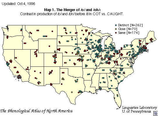
- Phonological Inventory: On a segmental level, the sound inventory used in the mental lexicon to represent the pronunciation of words can vary from speaker to speaker. For example most British English accents differentiate the words "cart", "cot" and "caught" using three different back open vowel qualities; however many American English accents use only two vowels in the three words (i.e. "cot" and "caught" become homophones). Similarly, older speakers of English may differentiate the word "poor" from the word "paw" through the use of a [ʊə] diphthong that is not used by younger speakers.
- Lexical Distribution: Even for the same phonological inventory, there may be distributional differences in terms of which segments are used in which words. For example, Northern and Southern varieties of British English differ in the selection of /ɑː/ and /æ/ in words like "bath", or differ in the selection of /ʌ/ and /ʊ/ in words like "strut". "Rhotic" accents articulate postvocalic /r/ in words like "farm".
- Allophonic variation: variations can occur in terms of the choice and distribution of allophones, for example the use of clear and dark variants of /l/, the replacement of syllablefinal /t/ with [ʔ], or the use of the labiodental approximant [ʋ] for /r/.
- Segmental quality: most clearly, accents vary in the precise articulatory implementation of the same phonemes, particularly vowels. The Northern Irish English realisation of the phoneme /aʊ/ is more like [ɑə] than the RP variant [ɐʊ]. Vowels not only vary in timbre, but can shift between monophthongs and diphthongs, the Geordie /əʊ/ can take the form [oː], or the London /i:/ as [ɪi].
- Prosody: variations also exist in prosody, in terms of lexical stress, timing and intonation. For example British English "adult" as /ˈædʌlt/ vs. American English /əˈdʌlt/; Southern English [baːd] vs Northern [bad]; or the use of the High-Rising Terminal intonation pattern ("uptalk") in statements in Northern Ireland
British English accent variation
A list of the major variations in British English is given in Hughes, Trudgill & Watt, 2005:
Variation Example Vowel /ʌ/ merge "butter" as /bʌtə/, /bʊtə/ Vowels /æ/ and /ɑ/ "laugh" as /læf/, /lɑːf/ Vowels /ɪ/ and /i/ "city" as /sɪtɪ/, /sɪti/ Post vocalic /r/ "farm" as /fɑːm/, /fɑːrm/ Vowels /ʊ/ and /uː/ "pull" as /pʊl/, /puːl/ /h/ dropping "harm" as /hɑːm/, /ɑːm/ Glottal stop [ʔ] "button" as [bʌtən], [bʌʔən] Velar nasal /ŋ/ "walking" as /wɔːkɪŋ/, /wɔːkɪn/ /j/ dropping "news" as /njuːz/, /nuːz/ lonɡ mid diphthonɡs "boat" as [bəʊt], [bɔːt] Second language accent variation
Another significant area of research is related to the accent of non-native speakers of a language. Typically the phonetic and phonological properties of a speaker's first language is seen to influence their pronunciation of a second language, particularly if that is learned later in life.
In this area of study, open questions include: whether it is possible to predict which sounds will be problematic knowing the phonology of the two languages, whether the problems arise from problems in perception, whether an ability to learn a native-like pronunciation worsens with age.
The problem for learners is not necessarily that new languages have new sounds. In the paper by Flege (see reading), English speakers were tested on their ability to produce French [u] and [y]. It turned out that [y] was different enough to any English vowel category that they produced that vowel with the same formant frequencies as French speakers. However the English speakers persevered with their English /u/ quality even if it was not the same as the French /u/ - that is they put the French [u] sound into the English /u/ category. Likewise English speakers productions of French /t/ had the long VOT of English [tʰ], not the short VOT of unaspirated [d̥] of French. Flege argues that learners cope with well exotic sounds but make mistakes when they re-use their L1 categories inappropriately for similar sounds.
Particularly well known examples of second-language accent problems include the difficulty of Japanese speakers to differentiate English /l/ and /r/ (perhaps because in Japanese these are heard as two allophones of the same phoneme). Conversely, English speakers may use a retroflex alveolar approximant [ɹ] for the French uvular approximant phoneme /ʁ/.
Finally
It may be worth pointing out that much accent variation is only detectable if one also knows what was said. Accents are characterised not so much by new sounds such as the same sounds in different places. The implication is that accents can only be recognised well from realisations of known utterances rather than from global properties of the speech.
- Quantification by counting
Historically, much work in accents has been undertaken by phoneticians with an ear for the varieties that people use. To identify what accents exist and their distribution across regions and social classes, a common approach would be to count the frequency of pronunciation variants as a function of indexical variables. For example, the sociolinguist Labov (1966) studied the frequency of use of post-vocalic /r/ and the frequency of use of [d] for /ð/ in different socio-economic groups in New York:
% use post-vocalic /r/ /ð/ as [d] Middle class 25 17 Working class 13 45 Lower class 11 56 To determine whether differences in counts could have arisen by chance, the chi-square statistic can be used. The relationships between frequencies and indexical variables can also be studied by means of clustering and principal components analysis. These examples taken from Stuart-Smith, Timmins & Tweedie (2007) in their study of differences in the Glaswegian accent across social classes.
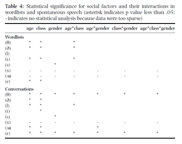
Significance of differences in relative frequency of occurrence of allophonic variants among factors of age, class and gender.
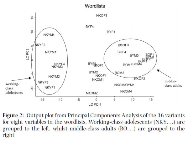
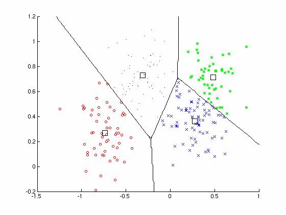
Principal components analysis places soocial groups on two dimensions on basis of eight dependent variables.
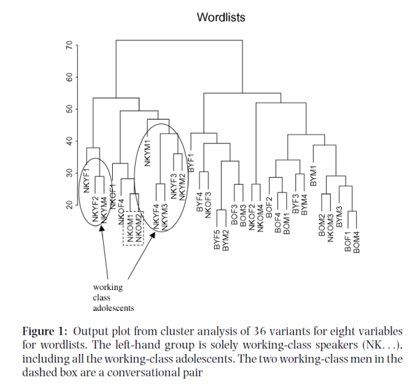
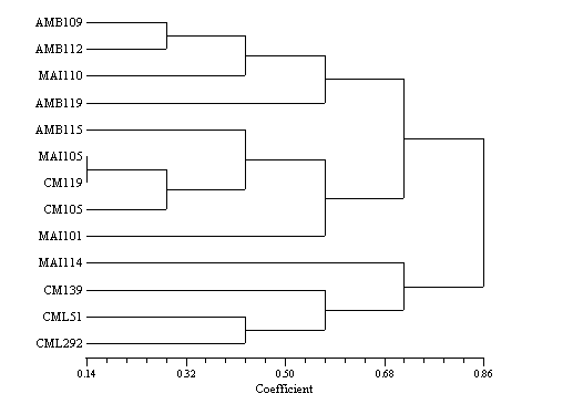
Clustering analysis shows hierarchichal relationship between social groups on basis of eight dependent variables.
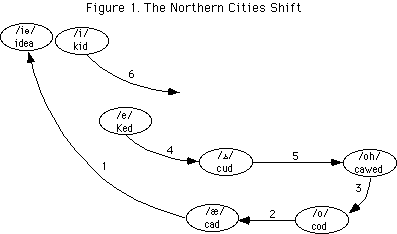
Another means of reporting accent variation is through the use of maps, such as Labov's study of "Cot-Caught" merger in North America:
Or graphical displays of accent change:
W. Labov, Principles of Linguistic Change Vol1: Internal Factors, 1994. W. Labov, Principles of Linguistic Change Vol2: Language in Society, 2001
- Quantification by acoustic measures
The availability of recorded speech materials has seen a shift towards instrumental measures of accent. Efforts have been concentrated on vowel formant frequencies, not only because vowels vary a great deal across accents, but also because vowels are easy to measure. As we have noted before, it is important to find a way to normalise formant frequencies before they can be compared across speakers. To ensure that measurements can be compared, the use of standardised materials (word/sentence lists) is essential. The Accents of the British Isles (ABI) corpus, and the Intonational varieties of English (IViE) corpus are good sources of materials for British English. Univariate and multivariate analysis of variance can be used to test the significance in shift of formant frequencies across groups.
Accent similarity metric
The availability of large, uniform corpora of spoken English makes possible new data-driven methods of accent discovery. The ACCDIST accent similarity metric (Huckvale, 2004) is a means to compare the pronunciation of two speakers saying the same utterances, without directly comparing the acoustic signals. Instead the similarity between segments within a speaker is used to create an inter-segment distance table, and the patterning in two such tables can then be correlated across speakers. The assumption is that similar accents will have similar distances between segments. For example, here are the table of distances between the 'a' vowel in "after", "father", and "cat" for two accents:
Since ACCDIST does not compare acoustic properties across speakers, no normalisation procedure is required. This also means that it can be used with spectral envelope features and be applied to consonants as well as vowels. ACCDIST has been shown to have superior performance for accent recognition compared to formant-based methods. Recent work has shown how ACCDIST can be applied to second language accents to predict the mutual intelligibility of L2 speakers.Birmingham South-east Distance father cat Distance father cat after 3.48 2.14 after 2.27 3.21 father 0.00 3.62 father 0.00 3.71 Accent Recognition Systems
Automatic systems for identifying accents are becoming more common. There are a number of basic strategies:
- Global spectral signature: compute summative statistics of spectral shape to describe a recorded passage, followed by a classification system.
- Statistical modelling of short-term spectral characteristics: use Gaussian Mixture Models to estimate the probability of an accent given a recording, in an anologus way to speaker recognition systems.
- Phone sequence modelling: collect statistics of phone frequency and phone sequence frequency at the output of a speech recogniser. Different accents would be expected to generate different sequence probabilities.
- Linguistic-Phonetic analysis: using text-dependent methods like ACCDIST.
Pubished performance figures for of accent recognition systems on the Accents of the British Isles corpus can be found in Hanani et al (2013):
System Description Accuracy % GMM recognition 61.13 GMM with classifier 76.11 Phonotactic 82.14 Combined GMM+Phonotactic 89.96 ACCDIST using correlation 93.17 ACCDIST with classifier 95.18 - Clustering
Since accents are properties of groups of speakers, clustering methods are convenient means for discovery of structure in measurement data. There are two main approaches to clustering: those that require a given number of clusters in advance, and those that produce a hierarchical analysis. If the number of clusters is known, then "k-means" clustering finds the identity of k centroids in the data, such that the total sum-squared distance of data vectors from their cluster centroids is minimised.
Agglomerative hierarchical clustering starts with all individual data vectors, then merges them in pairs until all are merged into one group. The ordering of the merge operations is displayed as a dendrogram, which can highlight sub-groups within the data.
Hierarchical Clustering with ACCDIST
The application of hierarchical clustering to accents was demonstrated in Huckvale (2007), as described below.
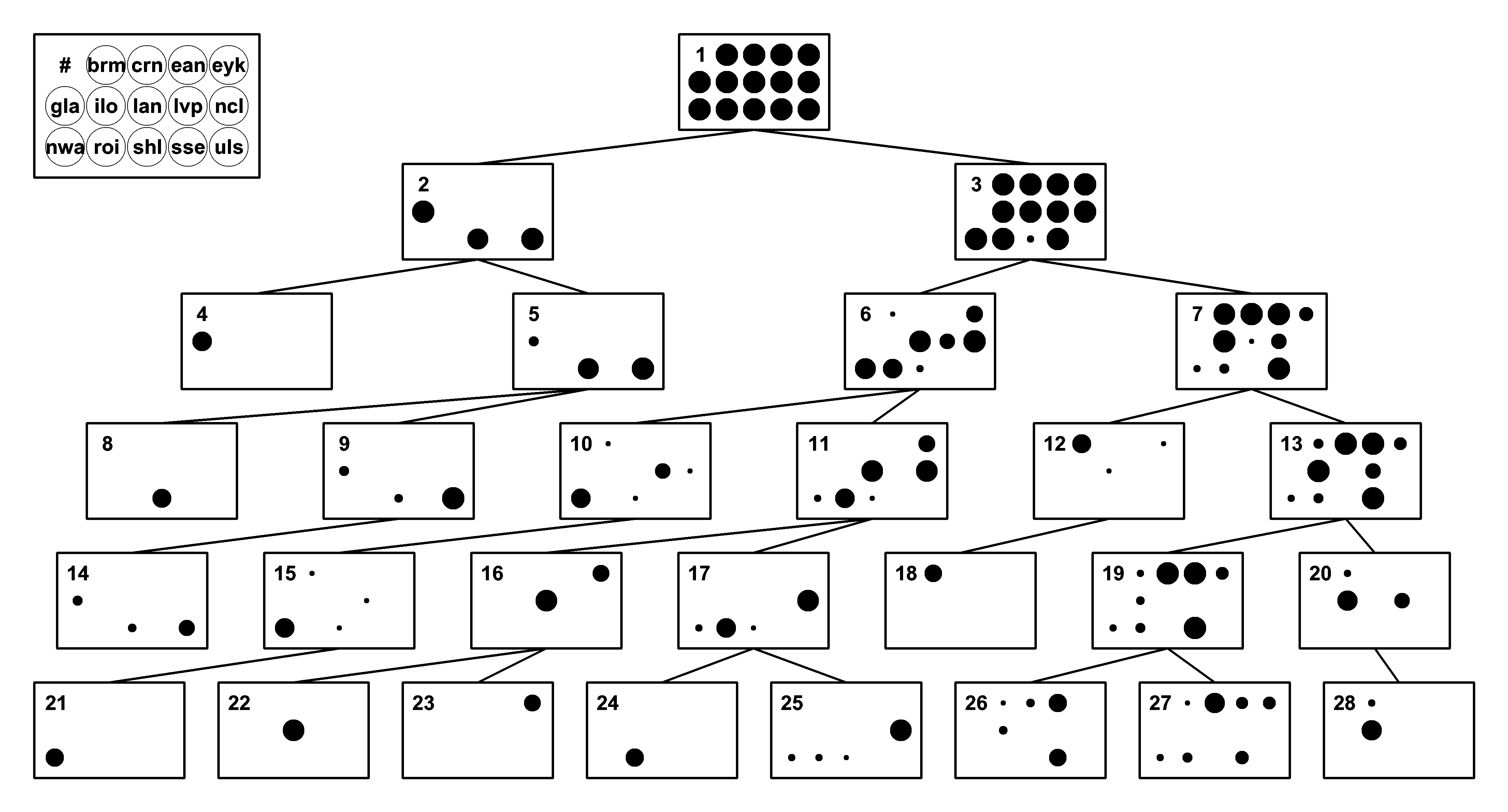
The diagrams compare two approaches to agglomerative hierarchical clustering of 275 speakers analysed by originating accent group. Each figure shows the top levels of a tree of 549 nodes. The area of the disks represents the proportion of the accent group members present in the node. For clarity, nodes which contain fewer than 10 speakers, or whose parent node consists entirely of speakers of one accent have been pruned. Accents codes are: brm=Birmingham, lvp=Liverpool, crn=Cornwall, ncl=Newcastle, ean=East Anglia, nwa=North Wales, eyk=East Yorkshire, roi=Dublin, gla=Glasgow, shl=Scottish Highlands, ilo=Inner London, sse=South East, lan=Lancashire, uls=Ulster.
(a) Clustering using a correlation measure on 2 raw formant frequencies and the complete linkage method. Accent purity=0.508. Note how the tree is unbalanced, with the bulk of the speakers in a single node even at the fourth tier of the tree.
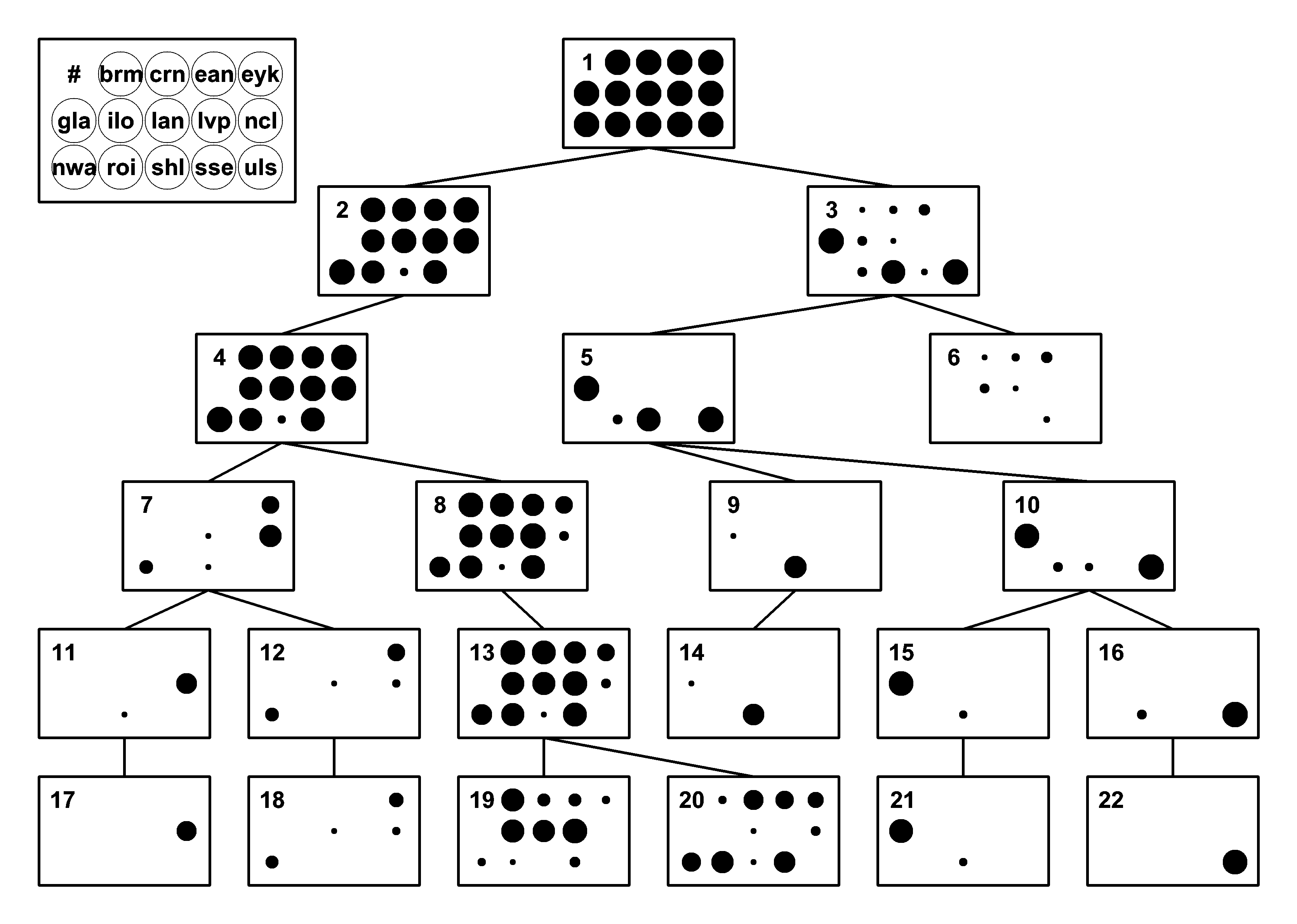
(b) Clustering using the ACCDIST measure on 13 spectral envelope features and the complete linkage method. Accent purity=0.647. Note how this tree is more balanced than (a), and how accent groups combine more cleanly. Interesting analyses can be made based on which accent groups cluster together at the highest levels.
References
- A. Hughes, P. Trudgill, D. Watt, English Accents and Dialects, Hodder Education, 2005, fourth edition.
- S. D'Arcy, M. Russell, S. Browning, M. Tomlinson, "The Accents of the British Isles (ABI), corpus", Proc. MIDL, Paris, 2004, 115-119.
- M. Huckvale, "ACCDIST: a metric for comparing speakers' accents", Proc. International Conference on Spoken Language Processing, Jeju, Korea, 2004.
- The IViE Corpus, English intonation in the British Isles, http://www.phon.ox.ac.uk/files/apps/IViE/index.php
- A. Hanani, M.J. Russell and M.J. Carey, "Human and computer recognition of regional accents and ethnic groups from British English speech", Computer Speech & Language 27 (2013) 59-74.
Readings
- M. Huckvale, "Hierarchical clustering of speakers into accents with the ACCDIST metric", Int. Congress of Phonetic Sciences, Saarbrucken, Germany, 2007.
- J. Stuart Smith, C. Timmins, F. Tweedie, "Talking Jockney? Variation and change in Glaswegian English", J. Sociolinguistics 11 (2007) 221-260.
- Jim Flege, "The production of 'new' and 'similar' phones in a foreign language: Evidence for the effect of equivalence classification". Journal of Phonetics, 15 (1987), 47-65.
Laboratory Exercise
- Two tables of formant frequencies extracted from student recordings are provided:
- y:\EP\vowform.csv: Mean F1 & F2 frequencies of 9 vowels from class recordings of the BKB sentences.
- y:\EP\vownorm.csv: Normalised mean F1 & F2 frequencies of the 9 vowels in z-scores w.r.t. to speaker average.
- Perform hierarchical clustering of speakers on the basis of the vowel measures using SPSS. Here are some basic instructions:
- Load the data set into SPSS, ensuring you specify that variable names are included at the top of the file.
- Run Analyze|Classify|Hierarchical Cluster
- Put ID into "Label cases by", and all the other variables into "Variables".
- On the "Statistics" option, request "Range of solutions" from 2 to 5.
- On the "Plots" option, request a "Dendrogram", and a "Horizontal" icicle plot.
- On the "Method" option, choose the "Transform Values" option depending on the data set. For "vowform.txt" select "Standardize:Z scores", while for "vownorm.txt", select "Standardize:None". The "Cluster Method" should be set to "Between-groups" and the "Measure" should be set to "Squared Euclidean" (default).
- Run the analysis.
- Print out and compare the clustering results obtained for the two data files. Can you find any interpretation for the clustering? What effect does the normalisation have?
- A table of accent similarities can be found y:\EP\distmeanaccent.sav. These have been computed using 20 speakers of 14 accent areas of the British Isles using the ACCDIST metric and are based on MFCC parameters from vowels alone. The accents are coded as follows:
- Load this file into SPSS. The 14 "VAR" columns are the similarities between accents expressed as correlation coefficients. You can input these directly into hierarchical clustering in SPSS with the command:
- A table of accent similarities between class speakers can be found in y:\EP\distspeaker.sav. These were computed using the ACCDIST metric applied to an MFCC analysis of vowels in the class BKB sentence recordings. Perform a similar clustering analysis as in 5. and interpret the clusters. Compare with the clustering you found in 3.
| Code | Accent | Code | Accent |
|---|---|---|---|
| brm | Birmingham | lvp | Liverpool |
| crn | Cornwall | ncl | Newcastle |
| ean | East Anglia | nwa | North Wales |
| eyk | East Yorkshire | roi | Dublin |
| gla | Glasgow | shl | Scottish Highlands |
| ilo | Inner London | sse | South East |
| lan | Lancashire | uls | Ulster |
CLUSTER
   /MATRIX=IN(*)
   /METHOD BAVERAGE
   /ID=Name
   /PRINT SCHEDULE
   /PLOT DENDROGRAM HICICLE(2,4,1).
Use New|Syntax to open a command window in SPSS to enter and run this command. Analyze how SPSS has clustered the accents.
Reflections
- Why is RP considered a non-regional accent?
- What would happen if you clustered speakers using un-normalised vowel formant frequencies?
- Why might a Northern English speaker accidentally pronounce "pasta" as /pɑːstə/?
- Why do accents change over time?
Word count: . Last modified: 09:53 16-Mar-2017.